Quantcast
Channel: Roland Bouman's blog
Viewing all 76 articles
Browse latest View live

Fighting Spam: Word Verification

$
0
0
Hi All,

this is a quick note to let you know that from now on, commenters on this blog will need to complete a word verification (captcha) step.

Personally, I regret to have to take this measure. Let me explain why I'm doing it anyway.

Since 3 months or so, moderating comments on this blog is becoming a real drag due to a surge in anonymous spam. While bloggers spam detection is quite good, I still get notificaton mails prompting me to moderate. I feel this is consuming more of my time than it's worth.

Except for requiring word verification, other policies (or lack thereof) are still in effect: all comments are moderated, but anyone can comment, even anonymously. In practice, all real comments get published - even negative or derogatory ones (should I receive them).

Sorry for the convenience, but I hope you'll understand.

MySQL Hacks: Preventing deletion of specific rows

$
0
0
Recently, someone emailed me:
I have a requirement in MYSQL as follows:
we have a table EMP and we have to restrict the users not delete employees with DEPT_ID = 10. If user executes a DELETE statement without giving any WHERE condition all the rows should be deleted except those with DEPT_ID = 10.

We are trying to write a BEFORE DELETE trigger but we are not able to get this functionality.

I have seen your blog where you explained about Using an UDF to Raise Errors from inside MySQL Procedures and/or Triggers. Will it helps me to get this functionality? Could you suggest if we have any other alternatives to do this as well?
Frankly, I usually refer people that write me these things to a public forum, but this time I felt like giving it a go. I figured it would be nice to share my solution and I'm also curious if others found other solutions still.

(Oh, I should point out that I haven't asked what the underlying reasons are for this somewhat extraordinary requirement. I normally would do that if I would be confronted with sucha a requirement in a professional setting. In this case I'm only interested in finding a crazy hack)

Attempt 1: Re-insert deleted rows with a trigger

My first suggestion was:
Raising the error won't help you achieve your goal: as soon as you raise the error, the statement will either abort (in case of a non-transactional table) or rollback all row changes made up to raising the error (in case of a transactional table)

Although I find the requirement strange, here's a trick you could try:

write a AFTER DELETE FOR EACH ROW trigger that re-inserts the rows back into the table in case the condition DEPT_ID = 10 is met.

Hope this helps...

Alas, I should've actually tried it myself before replying, because it doesn't work. If you do try it, a DELETEresults in this runtime error:
Can't update table 'emp' in stored function/trigger because it is already used by statement which invoked this stored function/trigger.
This is also known as "the mutating table problem".

Attempt 2: Re-insert deleted rows into a FEDERATED table

As it turns out, there is a workaround that meets all of the original demands. The workaround relies on the FEDERATED storage engine, which we can use to trick MySQL into thinking we're manipulating a different table than the one that fires the trigger. My first attempt went something like this:

CREATE TABLE t (
id INT AUTO_INCREMENT PRIMARY KEY,
dept_id INT,
INDEX(dept_id)
);

CREATE TABLE federated_t (
id INT AUTO_INCREMENT PRIMARY KEY,
dept_id INT,
INDEX(dept_id)
)
ENGINE FEDERATED
CONNECTION = 'mysql://root@localhost:3306/test/t';

DELIMITER //

CREATE TRIGGER adr_t
AFTER DELETE ON t
FOR EACH ROW
IF old.dept_id = 10 THEN
INSERT INTO t_federated
VALUES (old.id, old.dept_id);
END IF;
//

DELIMITER ;
So the idea is to let the trigger re-insert the deleted rows back into the federated table, which in turn points to the original table that fired the trigger to fool MySQL into thinking it isn't touching the mutating table. Although this does prevent one from deleting any rows that satisfy the DEPT_ID = 10 condition, it does not work as intended:

mysql> INSERT INTO t VALUES (1,10), (2,20), (3,30);
Query OK, 3 rows affected (0.11 sec)

mysql> DELETE FROM t;
ERROR 1159 (08S01): Got timeout reading communication packets

mysql> SELECT * FROM t;
+----+---------+
| id | dept_id |
+----+---------+
| 1 | 10 |
| 2 | 20 |
| 3 | 30 |
+----+---------+
3 rows in set (0.00 sec)
At this point I can only make an educated guess about the actual underlying reason for this failure. It could be that the deletion is locking the rows or even the table, thereby blocking the insert into the federated table until we get a timeout. Or maybe MySQL enters into an infinite loop of deletions and insertions until we hit a timeout. I didn't investigate, so I don't know, but it seems clear this naive solution doesn't solve he problem.

Attempt 3: Deleting from the FEDERATED table and re-inserting into the underlying table

It turns out that we can solve it with a FEDERATED table by turning the problem around: Instead of manipulating the original table, we can INSERT and DELETE from the FEDERATED table, and have an AFTER DELETE trigger on the FEDERATED table re-insert the deleted rows back into the original table:

DROP TRIGGER adr_t;

DELIMITER //

CREATE TRIGGER adr_federated_t
AFTER DELETE ON federated_t
FOR EACH ROW
IF old.dept_id = 10 THEN
INSERT INTO t
VALUES (old.id, old.dept_id);
END IF;
//

DELIMITER ;
Now, the DELETE does work as intended:

mysql> DELETE FROM federated_t;
Query OK, 3 rows affected (0.14 sec)

mysql> SELECT * FROM federated_t;
+----+---------+
| id | dept_id |
+----+---------+
| 1 | 10 |
+----+---------+
1 row in set (0.00 sec)
Of course, to actually use this solution, one would grant applications access only to the federated table, and "hide" the underlying table so they can't bypass the trigger by deleting rows directly from the underlying table.

Now, even though this solution does seem to fit the original requirements, I would not recommend it for several reasons:
  • It uses the FEDERATED storage engine, which hasn't been well supported. For that reason, it isn't enabled by default, and you need access to the MySQL configuration to enable it, limiting the applicability of this solution. Also, you could run into some nasty performance problems with the FEDERATED storage engine
  • The solution relies on a trigger. In MySQL, triggers can really limit performance
  • Perhaps the most important reason is that this solution performs "magic" by altering the behaviour of SQL statements. Arguably, this is not so much the fault of the solution as it is of the original requirement.

An Alternative without relying on magic: a foreign key constraint

If I were to encounter the original requirement in a professional situation, I would argue that we should not desire to alter the semantics of SQL commands. If we tell the RDBMS to delete all rows from a table, it should either succeed and result in all rows being deleted, or it should fail and fail completely, leaving the data unchanged.

So how would we go about implementing a solution for this changed requirement?

We certainly could try the approach that was suggested in the original request: create a trigger that raises an exception whenever we find the row should not be deleted. However, this would still rely on a trigger (which is slow). And if you're not on MySQL 5.5 (or higher), you would have to use one of the ugly hacks to raise an exception.

As it turns out, there is a very simple solution that does not rely on triggers. We can create a "guard table" that references the table we want to protect using a foreign key constraint:

mysql> CREATE TABLE t_guard (
-> dept_id INT PRIMARY KEY,
-> FOREIGN KEY (dept_id)
-> REFERENCES t(dept_id)
-> );
Query OK, 0 rows affected (0.11 sec)

mysql> INSERT INTO t_guard values (10);
Query OK, 1 row affected (0.08 sec)

mysql> DELETE FROM t;
ERROR 1451 (23000): Cannot delete or update a parent row: a foreign key constraint fails (`test`.`t_guard`, CONSTRAINT `t_guard_ibfk_1` FOREIGN KEY (`dept_id`) REFERENCES `t` (`dept_id`))
mysql> DELETE FROM t WHERE dept_id != 10;
Query OK, 2 rows affected (0.05 sec)
(Like in the prior example with the federated table, the guard table would not be accessible to the application, and the "guard rows" would have to be inserted by a privileged user)

Finally: what a quirkyy foreign key constraint!

You might have noticed that there's something quite peculiar about the foreign key constraint: typically, foreign key constraints serve to relate "child" rows to their respective "parent" row. To do that, the foreign key would typically point to a column (or set of columns) that make up either the primary key or a unique constraint in the parent table. But in this case, the referenced column dept_id in the t table is contained only in an index which is not unique. Strange as it may seem, this is allowed by MySQL (or rather, InnoDB). In this particular case, this flexibility (or is it a bug?) serves us quite well, and it allows us to guard many rows in the t table with dept_id = 10 with just one single row in the guard table.

Common Schema: dependencies routines

$
0
0
Are you a MySQL DBA? Checkout the common_schema project by Oracle Ace Shlomi Noach.

The common_schema is an open source MySQL schema that packs a number of utility views, functions and stored procedures. You can use these utilities to simplify MySQL database administration and development. Shlomi just released revision 178, and I'm happy and proud to be working together with Shlomi on this project.

Among the many cool features created by Shlomi, such as foreach, repeat_exec and exec_file, there are a few %_dependencies procedures I contributed:

  • get_event_dependencies(schema_name, event_name)

  • get_routine_dependencies(schema_name, routine_name)

  • get_sql_dependencies(sql, default_schema)

  • get_view_dependencies(schema_name, view_name)

All these procedures return a resultset that indicates which schema objects are used by the object identified by the input parameters. Here are a few examples that should give you an idea:

mysql> call common_schema.get_routine_dependencies('common_schema', 'get_routine_dependencies');
+---------------+----------------------+-------------+--------+
| schema_name | object_name | object_type | action |
+---------------+----------------------+-------------+--------+
| common_schema | get_sql_dependencies | procedure | call |
| mysql | proc | table | select |
+---------------+----------------------+-------------+--------+
2 rows in set (0.19 sec)

Query OK, 0 rows affected (0.19 sec)

mysql> call common_schema.get_routine_dependencies('common_schema', 'get_sql_dependencies');
+---------------+-------------------+-------------+--------+
| schema_name | object_name | object_type | action |
+---------------+-------------------+-------------+--------+
| common_schema | _get_sql_token | procedure | call |
| common_schema | _sql_dependencies | table | create |
| common_schema | _sql_dependencies | table | drop |
| common_schema | _sql_dependencies | table | insert |
| common_schema | _sql_dependencies | table | select |
+---------------+-------------------+-------------+--------+
5 rows in set (1.59 sec)
Of course, there's always a lot to be desired. The main shortcomings as I see it now is that the dependencies are listed only one level deep: that is, the dependencies are not recursively analyzed. Another problem is that there is currently nothing to calculate reverse dependencies (which would arguably be more useful).

The good news is, this is all open source, and your contributions are welcome! If you're interested in the source code of these routines, checkout the common_schema project, and look in the common_schema/routines/dependencies directory.

If you'd like to add recursive dependencies, or reverse dependencies, then don't hesitate and contribute. If you have a one-off contribution that relates directly to these dependencies routines, then it's probably easiest if you email me directly, and I'll see what I can do to get it in. If you are interested in more long term contribution, it's probably best if you write Shlomi, as he is the owner of the common_schema project.

You can even contribute without implementing new features or fixing bugs. You can simply contribute by using the software and find bugs or offer suggestions to improve it. If you found a bug, or have an idea for an improvement or an entirely new feature, please use the issue tracker.

For now, enjoy, and untill next time.

Running Pentaho BI Server behind a proxy

$
0
0
To whom it may concern - a quick hands-on guide for running the Pentaho BI server behind a proxy

Prerequisites


This post assumes you're running Ubuntu linux (or at least a Debian) and that you have both the apache Httpd server as well as the Pentaho BI server installed.

Apache HTTP Server


If you haven't got apache installed, this is your line:
$ sudo apt-get install apache2

You can then control the apache2 Http server using the apaceh2ctl script. For instance, to start it, do:
$ sudo apache2ctl start

Once it's started you can navigate to its homepage to verify that it is running:
http://localhost/

You can stop it by running
$ sudo apache2ctl stop

If you're changing apache's configuration, you need to restart it to allow changes to take effect using this command:
$ sudo apache2ctl restart
.

Java


Pentaho relies on Java. If not installed already you can get it like this:
$ sudo apt-get install openjdk-6-jdk

Pentaho BI Server


If you haven't got the Pentaho BI Server, download the latest version from sourceforge, and unpack the archive in some location you find convenient. (For development purposes I simply keep and run it in a subdirectory of my home directory)

You can start the pentaho BI Server by cd-ing into the biserver-ce directory and then run:
$ ./start-pentaho.sh

You can then navigate to its homepage:
http://localhost:8080/pentaho/Home

(Simply navigating to http://localhost:8080 will automatically redirect you there too).

It can be useful to monitor the log while it's running:
$ tail -f tomcat/logs/catalina.out

If you want to change something in Pentaho's configuration, you need to stop the server and then restart it. This is done by running:
$ ./stop-pentaho.sh

Configuring Proxy support for Apache


Boris Kuzmanovic wrote an excellent post to setting up proxy support for Apache. My summary (and adjustment) follows below.

First, change the apache configuration to load the required proxy modules:
$ sudo a2enmod proxy
$ sudo a2enmod proxy_http

Then, edit any site definitions to use the proxy. I just modified the default site definition:
$ sudo geany /etc/apache2/sites-enabled/000-default


Inside the <VirtualHost> section, I added these snippets immediately above the </VirtualHost> that ends the section:

<Location /pentaho/>
ProxyPass http://localhost:8080/pentaho/
ProxyPassReverse http://localhost:8080/pentaho/
SetEnv proxy-chain-auth
</Location>

<Location /pentaho-style/>
ProxyPass http://localhost:8080/pentaho-style/
ProxyPassReverse http://localhost:8080/pentaho-style/
SetEnv proxy-chain-auth
</Location>


After making these changes, we need to restart apache:
$ sudo apache2ctl restart
.

These two <Location> directives are now effectively tunneled to the respective locations on the Pentaho BI Server, and vice versa, the response is passed back.

Using mod_proxy_ajp instead of proxy_http


While the regular HTTP proxy simply works, there is a better, more thightly integrated solution. The regular HTTP proxy basically handles HTTP requests received by the Apache Httpd server by sending a new, equivalent HTTP request, through to the tomcat server. Likewise, Tomcat's HTTP response is then send back as a new equivalent HTTP response to the source of the original, initial request.

So, that's twice a transport over HTTP.

Things can be improved by routing the incoming HTTP request to the tomcat server using a binary protocol called the AJP (Apache JServ) protocol. (For a detailed comparison, see this excellent comparison between HTTP/HTTPS and AJP.)

Fortunately, the steps to setup an AJP proxy are almost identical to those for setting up a regular HTTP proxy. First, enable the ajp proxy module:
$ sudo a2enmod proxy
$ sudo a2enmod proxy_ajp

(Note that the proxy module was already enabled as part of setting up the regular http proxy. The line is repeated here for completeness, but not necessary if you completed the steps for setting up support for the regular http proxy. You can enable either or both the proxy_http and the proxy_ajp modules, and both require the proxy module.)

Then, we edit again the site configuration to use the proxy. Since the locations /pentaho/ and /pentaho-style/ were already used, we first comment those out:

#<Location /pentaho/>
# ProxyPass http://localhost:8080/pentaho/
# ProxyPassReverse http://localhost:8080/pentaho/
# SetEnv proxy-chain-auth
#</Location>

#<Location /pentaho-style/>
# ProxyPass http://localhost:8080/pentaho-style/
# ProxyPassReverse http://localhost:8080/pentaho-style/
# SetEnv proxy-chain-auth
#</Location>


Then we add equivalent lines going via the AJP proxy:

ProxyPass /pentaho ajp://localhost:8009/pentaho
ProxyPassReverse /pentaho ajp://localhost:8009/pentaho

ProxyPass /pentaho-style ajp://localhost:8009/pentaho-style
ProxyPassReverse /pentaho-style ajp://localhost:8009/pentaho-style

(The bit that goes ajp://localhost:8009 refers to the ajp service that is running on port 8009 of tomcat by default.)

Again we have to restart the apache service for the changes to take effect:
$ sudo apache2ctl restart
.

Acknowledgements


Thanks to Paul Stöllberger, Pedro Alves and Tom Barber for valuable feedback and background information regarding AJP.

A Generic Normalizer step for Kettle

$
0
0

Abstract

Kettle (a.k.a. Pentaho Data Integration) offers the standard Row Normalizer step to "unpivot" columns to rows. However, this step requires some configuration which presumes its input stream is static, and its structure is known. In this post, I explain how to construct a simple User-defined java class step that implements a generic Row Normalizer step that can unpivot an arbitrary input stream without manual configuration.

The Row Normalizer step


Kettle (a.k.a. Pentaho Data Integration) offers a standard step to "unpivot" columns to rows. This step is called the Row Normalizer. You can see it in action in the screenshot below:

In the screenshot, the input is a table of columns id, first name, and last name. The output is a table of columns id, fieldname, and value. The id column is preserved, but for each row coming from the input stream, two rows are created in the output stream: 1 for the first name field, and 1 for the last name field.

Essentially the Row Normalizer step in this example is configured to treat the first name and last name fields as a repeating group. The repeating group is untangled by dumping all values for either field in the value column. The fieldname column is used to mark the kind of value: some values are of the "first name field" kind (in case they came from the original first name input field), some are from the "last name field" kind (when the derive from the last name input field).

There are several use cases for the operation performed by the Row normalizer step. It could be used to break down a genuine repeating group in order to create a more normalized dataset. Or you might need to convert a relational dataset into a graph consisting of subject-predicate-object tuples for loading a triple store. Or maybe you want to turn a table into a fine-grained stream of changes for auditing.

The problem

The Row normalizer step works great for streams that have a structure that is known in advance. The structure needs to be known in advance in order to specify those fields that are to be considered as repeating group in the step configuration so they can be broken out into separate kinds.

Sometimes, you don't know the structure of the input stream in advance, or it is just to inconvenient to manually specify it. In these cases, you'd really wish you could somehow unpivot any field that happens to be part of the input stream. In other words, you'd need to have a generic Row Normalizer step.

The Solution

In Kettle, there's always a solution, and often more. Here, I'd like to present a solution to dynamically unpivot an arbitrary input stream using a user-defined java class step.

Below is a screenshot of the step configuration:

This configuration allows the step to take an arbitrary input stream and normalize it into a collection of triples consisting of:
  1. An id column. This column delivers generated integer values, and each distinct value uniquely identifies a single input row.
  2. A fieldnum column. This is a generated integer value that uniquely identifies a field within each input row.
  3. A value column. This is a string column that contains the value that appears in the field identified by the fieldnum column within the row identified by the rownum value.

The Row Normalizer versus the UJDC generic Normalizer

For the input data set mentioned in the initial example, the output generated by this UJDC step is shown below:
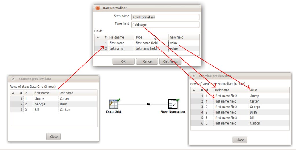
There are a few differences with regard to the output of kettle's Row Normalizer step:
  1. One obvious difference is that the Row Normalizer step has the ability to attach names to the values, whereas the UJDC step only delivers a generated field position. One the one hand, it's really nice to have field names. On the other hand, this is also one of the weaknesses of the Row Normalizer step, because providing the names most be done manually.
  2. Another difference is that the UDJC step delivers 3 output rows for each input row, instead of the 2 rows delivered by the Row Normalizer step. The "extra" row is due to the id column. Because the id column is the key of the original input data, the Row Normalizer step was configured to only unpivot the first name and last name fields, keeping the id field unscathed: this allows any downstream steps to see which fields belong to which row. The UDJC step however does not know which field or fields form the key of the input stream. Instead, it generates its own key, the rownum field, and the id field is simply treated like any other field and unpivoted, just like the first name and last name fields. So the main difference is that the downstream steps need to use the generated rownum field to see which fields belong to which row.

The Code

The code and comments are pretty straightforward:
static long rownum = 0;
static RowMetaInterface inputRowMeta;
static long numFields;
static String[] fieldNames;

public boolean processRow(StepMetaInterface smi, StepDataInterface sdi) throws KettleException
{
// get the current row
Object[] r = getRow();

// If the row object is null, we are done processing.
if (r == null) {
setOutputDone();
return false;
}

// If this is the first row, cache some metadata.
// We will reuse this metadata in processing the rest of the rows.
if (first) {
inputRowMeta = getInputRowMeta();
fieldNames = inputRowMeta.getFieldNames();
numFields = fieldNames.length;
}

// Generate a new id number for the current row.
rownum += 1;

// Generate one output row for each field in the input stream.
int fieldnum;
for (fieldnum = 0; fieldnum < numFields; fieldnum++) {
Object[] outputRow = new Object[3];
outputRow[0] = rownum;
// Assign the field id. Note that we need to cast to long to match Kettle's type system.
outputRow[1] = (long)fieldnum+1;
outputRow[2] = inputRowMeta.getString(r, fieldnum);
putRow(data.outputRowMeta, outputRow);
}

return true;
}

Getting Field information

So the UDJC step only generates a number to identify the field. For some purposes it may be useful to pull in other information about the fields, like their name, data type or data format. While we could do this also directly int the UDJC step by writing more java code, it is easier and more flexible to use some of Kettle's built-in steps:
  1. The Get Metadata Structure step. This step takes an input stream, and generates one row for each distinct field. Each of these rows has a number of columns that describe the field from the input stream. One of the fields is a Position field, which uniquely identifies each field from the input stream using a generated integer, just like the fieldnum field from our UJDC step does.
  2. The stream lookup step. This step allows us to combine the output stream of our UJDC step with the output of the Get Metadata structure step. By matching the Position field of the Get Metadata Structure step with the fieldnum field of the UDJC step, we can lookup any metadata fields that we happen to find useful.


Below is a screenshot that shows how all these steps work together:
And here endeth the lesson.

When kettle's "Get data From XML" is bombed by the BOM

$
0
0
To whom it may concern...
I just ran into a problem with Pentaho Data Integration, and I figured it may save others some time if I document it here.
The case is very straightforward: read a fairly small XML document directly from a URL, and parse out interesting data using the Get data from XML step.
Typically, this steps works quite well for me. But I just ran into a case where it doesn't work quite as expected. I ran into an error when I tried it on this URL:

http://api.worldbank.org/en/countries?page=1
If you follow the URL you'll find it returns a normal looking document:

<?xml version="1.0" encoding="utf-8"?>
<wb:countries page="1" pages="6" per_page="50" total="260" xmlns:wb="http://www.worldbank.org">
<wb:country id="ABW">
<wb:iso2Code>AW</wb:iso2Code>
<wb:name>Aruba</wb:name>
<wb:region id="LCN">Latin America &amp; Caribbean (all income levels)</wb:region>
<wb:adminregion id="" />
<wb:incomeLevel id="NOC">High income: nonOECD</wb:incomeLevel>
<wb:lendingType id="LNX">Not classified</wb:lendingType>
<wb:capitalCity>Oranjestad</wb:capitalCity>
<wb:longitude>-70.0167</wb:longitude>
<wb:latitude>12.5167</wb:latitude>
</wb:country>
...
</wb:countries>

The error: Content is not allowed in prolog

The error I got was:

Content is not allowed in prolog.
You can encounter this error in any context where the step tries to retrieve the document from the URL, for example when you hit the "Get XPAth nodes" or "Preview" buttons, as well as when you're actually running the step.

Using the w3c XML validator

The error message indicates that the XML document is in some way not valid. So I ran the URL through the w3c validator:

http://validator.w3.org/check?uri=http%3A%2F%2Fapi.worldbank.org%2Fen%2Fcountries%3Fpage%3D1&charset=%28detect+automatically%29&doctype=Inline&group=0
Interestingly, this indicated that the document is valid XML.

A rather dismal workaround

Then I tried a few things in kettle in an attempt to work around it. I won't bother you with everything I tried. Eventually, I did find a viable work-around: By retrieving the document with the HTTP Client step, and then saving that to file using a simple Text file output step (omitting the header, separators, and quotes), I could then successfully open and parse that file with the "Get data from XML" step (from within a second transformation). This was of course a bit annoying since it involved a second transformation, which complicates things considerably. However all attempts to skip the "Text file output" step all brought me back to where I was and gave me the dreaded Content is not allowed in prolog. error. So something was happening to the document between saving and loading from disk that somehow fixed it.

Mind w3c validator Warnings!

I decided to investigate a bit more. What I didn't notice at first when I validated the XML document is that, despite passing validation, it does yield 2 warnings:
  • No DOCTYPE found! Checking XML syntax only.
  • Byte-Order Mark found in UTF-8 File.
As it turns out, this second warning conveys a very important tidbit of information.

UTF-8, the BOM, and java don't play nice together

I knew what a BOM was, but I didn't quite understand it's implications in particular for java and java-based applications. Here's a quick list of things you need to know to understand the problem:
  • The byte-order mark (BOM) is a special unicode character that indicates several details of the encoding of an inputstream.
  • The BOM is optional, and for UTF-8 it is actually disrecommended. But, apparently, this does not mean it's never there, or even non-standard!
  • The particular combination of a BOM occurring in a UTF-8 stream is not supported by java. There are bug reports about it here and here.
Maybe the Get data from XML step should be more forgiving, and take care of the BOM for us if it does occur. It sure would have saved me time. Anyway, it currently doesn't, and I came up with the following solution that is reasonably straightforward and does solve the problem:

A better workaround

We can first retrieve the document with the "Http Client" step, and then remove the BOM if it is present, and then process the document using the Get data from XML step. The transformation below illustrates that setup: So, the "HTTP client" step retrieves the XML text in the document field, and the User-defined Java Expression step simply finds the first occurrence of the less than character (<), which demarcates either the start of the xml declaration, or the document element. The code for that expression is rather straightforward:

document.substring(document.indexOf("<"))
All in all, not very pretty, but it does the job. I hope this was of some use to you.
UPDATE1: I created PDI-12410 pertaining to this case.
UPDATE2: Apart from the BOM, there seems to be a separate, independent problem when the XML is acquired from a URL and the server uses gzip compression.
UPDATE3: I have a commit here that solves both the BOM and the gzip issues: https://github.com/rpbouman/pentaho-kettle/commit/6cf28b5e4e88022dbf356ccad01c3b949bed4731.

MySQL: Extracting timstamp and MAC address from UUIDs

$
0
0
To whom it may concern.

Surrogate keys: auto-increment or UUID?

I recently overheard a statement about whether to use auto-incrementing id's (i.e, a sequence managed by the RDBMS) or universal unique identifiers (UUIDs) as method for generating surrogate key values.

Leakiness

Much has been written about this subject with regard to storage space, query performance and so on, but in this particular case the main consideration was leakiness. Leakiness in this case means that key values convey information about the state of the system that we didn't intend to disclose.

Auto-incrementing id's are leaky

For example, suppose you would subscribe to a new social media site, and you get assigned a personal profile page which looks like this:

http://social.media.site/user/67638
Suppose that 67638 is the auto-incrementing key value that was uniquely assigned to the profile. If that were the case then we could wait a day and create a new profile. We could then compare the key values and use it to estimate how many new profiles were created during that day. This might not necessarily be very sensitive information, but the point here is that by exposing the key values, the system exposes information that it didn't intend to disclose (or at least not in that way).

Are UUIDs leaky?

So clearly, auto-incrementing keys are leaky. The question is, are UUIDs less leaky? Because if that's the case, then that might weigh in on your consideration to choose for a UUID surrogate key. As it turns out, this question can be answered with the universal but always unsatisfactory answer that "it depends". Not all UUIDs are created equal, and wikipedia lists 5 different variants. This is not an exhaustive list, since vendors can (and so, probably will) invent their own variants.

MySQL UUIDs

In this article I want to focus on MySQL's implementation. MySQL has two different functions that generate UUIDs: UUID() and UUID_SHORT().

Are MySQL UUIDs leaky?

If you follow the links and read the documentation, then we can easily give a definitive answer, which is: yes, MySQL UUIDs are leaky:It is not my role to judge whether this leakiness is better or worse than the leakiness of auto-incrementing keys, I'm just providing the information so you can decide whether it affects you or not.

Hacking MySQL UUID values

Now, on to the fun bit. Let's hack MySQL UUIDs and extract meaningful information. Because we can.

Credit where credit's due: Although the documentation and MySQL source code contain all the information, I had a lot of benefit from the inconspicuously-looking but otherwise excellent website from the Kruithof family. It provides a neat recipe for extracting timestamp and MAC address from type 1 UUIDs. Thanks!

Here's a graphical representation of the recipe:

Without further ado, here come the hacks:

Extracting the timestamp from a MySQL UUID

Here's how:

select uid AS uid
, from_unixtime(
(conv(
concat( -- step 1: reconstruct hexadecimal timestamp
substring(uid, 16, 3)
, substring(uid, 10, 4)
, substring(uid, 1, 8)
), 16, 10) -- step 2: convert hexadecimal to decimal
div 10 div 1000 div 1000 -- step 3: go from nanoseconds to seconds
) - (141427 * 24 * 60 * 60) -- step 4: substract timestamp offset (October 15,
) AS uuid_to_timestamp
, current_timestamp() AS timestamp
from (select uuid() uid) AS alias;
Here's an example result:

+--------------------------------------+---------------------+---------------------+
| uid | uuid_to_timestamp | timestamp |
+--------------------------------------+---------------------+---------------------+
| a89e6d7b-f2ec-11e3-bcfb-5c514fe65f28 | 2014-06-13 13:20:00 | 2014-06-13 13:20:00 |
+--------------------------------------+---------------------+---------------------+
1 row in set (0.01 sec)
The query works by first obtaining the value from UUID(). I use a subquery in the from clause for that, which aliases the UUID() function call to uid. This allows other expressions to manipulate the same uid value. You cannot simply call the UUID() multiple times, since it generates a new unique value each time you call it. The raw value of uid is shown as well, which is:a89e6d7b-f2ec-11e3-bcfb-5c514fe65f28. Most people will recognize this as 5 hexadecimal fields, separated by dashes. The first step is to extract and re-order parts of the uid to reconstruct a valid timestamp:
  • Characters 16-18 form the most significant part of the timestamp. In our example that's 1e3; the last 3 characters of the third field in the uid.
  • Characters 10-13 form the middle part timestamp. In our example that's f2ec; this corresponds to the second field
  • Characters 1-8 form the least significant part of the timestamp. In our example that's a89e6d7b; this is the first field of the uid.

Extracting the parts is easy enough with SUBSTRING(), and we can use CONCAT() to glue the parts into the right order; that is, putting the most to least significant parts of the timestamp in a left-to-right order. The hexadecimal timestamp is now 1e3f2eca89e6d7b.

The second step is to convert the hexadecimal timestamp to a decimal value. We can do that using CONV(hextimestamp, 16, 10), where 16 represents the number base of the hexadecimal input timestamp, and 10 represents the number base of output value.

We now have a timestamp, but it is in a 100-nanosecond resolution. So the third step is to divide so that we get back to seconds resolution. We can safely use a DIV integer division. First we divide by 10 to go from 100-nanosecond resolution to microseconds; then by 1000 to go to milliseconds, and then again by 1000 to go from milliseconds to seconds.

We now have a timestamp expressed as the number of seconds since the date of Gregorian reform to the Christian calendar, which is set at October 15, 1582. We can easily convert this to unix time by subtracting the number of seconds between that date and January 1, 1970 (i.e. the start date for unix time). I suppose there are nicer ways to express that, but 141427 * 24 * 60 * 60 is the value we need to do the conversion.

We now have a unix timestamp, and MySQL offers the FROM_UNIXTIME() function to go from unix time to a MySQL timestamp value.

Extracting the MAC address from a MySQL UUID

The last field of type 1 UUID's is the so-called node id. On BSD and Linux platforms, MySQL uses the MAC address to create the node id. The following query extracts the MAC address in the familiar colon-separated representation:

select uid AS uid
, concat(
substring(uid, 25,2)
, ':', substring(uid, 27,2)
, ':', substring(uid, 29,2)
, ':', substring(uid, 31,2)
, ':', substring(uid, 33,2)
, ':', substring(uid, 35,2)
) AS uuid_to_mac
from (select uuid() uid) AS alias;
Here's the result:

+--------------------------------------+-------------------+
| uid | uuid_to_mac |
+--------------------------------------+-------------------+
| 78e5e7c0-f2f5-11e3-bcfb-5c514fe65f28 | 5c:51:4f:e6:5f:28 |
+--------------------------------------+-------------------+
1 row in set (0.01 sec)
I checked on Ubuntu with ifconfig and found that this actually works.

What about UUID_SHORT()?

The UUID_SHORT() function is implemented thus:

(server_id & 255) << 56
+ (server_startup_time_in_seconds << 24)
+ incremented_variable++;
This indicates we could try and apply right bitshifting to extract server id and start time.

Since the server_id can be larger (much larger) than 255, we cannot reliably extract it. However, you can give it a try; assuming there are many mysql replication clusters with less than 255 nodes, and assuming admins will often use a simple incrementing number scheme for the server id. you might give it a try.

The start time is also easy to extract with bitshift. Feel free to post queries for that in the comments.

Conclusions

I do not pretend to present any novel insights here, this is just a summary of well-known principles. The most important take-away is that you should strive to not expose system implementation details. Surrogate key values are implementation details so should never have been exposed in the first place. If you cannot meet that requirement (or you need to compromise because of some other requirement) then you, as system or application designer should be aware of the leakiness of your keys. In order to achieve that awareness, you must have insight at the implementation-level of how the keys are generated. Then you should be able to explain, in simple human language, to other engineers, product managers and users, which bits of information are leaking, and what would be the worst possible scenario of abuse of that information. Without that analysis you just cannot decide to expose the keys and hope for the best.

MySQL 5.7.5: GROUP BY respects functional dependencies!

$
0
0
Today, Oracle announced the availability of the Development Milestone Release 15 of MySQL 5.7.5. The tagline for this release promises "Enhanced Database Performance and Manageability". That may sound rather generic, the actual list of changes and improvements is simply *huge*, and includes many items that I personally find rather exciting! Perhaps I'm mistaken but I think this may be one of the largest number of changes packed into a MySQL point release that I've witnessed in a long time. The list of changes includes improvements such as:
  • InnoDB improvements: Simplified tablespace recovery, support for spatial indexes, dynamic configuration of the innodb_buffer_pool_size parameter(!), more efficient creation and rebuilding of indexes ("sorted index build")
  • Several general improvements for spatial data, such as support for open polygons and functions to manipulate geohash values and GeoJSON documents
  • performance_schema additions and improvements, such as a new user_variables_by_thread table, addition of WORK_COMPLETED and WORK_ESTIMATED columns to the stage event tables, improvements to the wait event tables, instrumentation for InnoDB memory allocation in the memory summary tables.
  • Quite a bunch of optimizer improvements, such as better cost estimation for semi-join materialization, configurable cost model (by way of the mysql.server_cost and mysql.engine_cost system tables) and more exact index statistics.
  • Many improvements and additions that make replication more robust
  • A more sane default SQL mode and GROUP BY behaviour
This is very far from an exhaustive list; It really is not an exaggeration to say that there is much much more than I can cover here. Just see for yourself.

Now, one of the changes I'd like to highlight in this post is the improved GROUP BY support.

GROUP BY behavior before MySQL 5.7.5

More than 7 years ago, I wrote an article on this blog called Debunking GROUP BY Myths. The article is basically an explanation of the syntax and semantics of the SQL GROUP BY clause, with a focus on MySQL particular non-standard implementation.

Before MySQL 5.7.5, MySQL would by default always aggregate over the list of expressions that appear in the GROUP BY-clause, even if the SELECT-list contains non-aggregate expressions that do not also appear in the GROUP BY-clause. In the final resultset, MySQL would produce one of the available values for such non-aggregate expressions and the result would basically not be deterministic from the user's point of view.

This behavior is not standard: SQL92 states that any non-aggregate expressions appearing in the SELECT-list must appear in the GROUP BY-clause; SQL99 and on state that any non-aggregate expressions that appear in the SELECT-list must be functionally dependent upon the list of expressions appearing in the GROUP BY. In this context, "functionally dependent" simply means that for each unique combination of values returned by the expressions that make up the GROUP BY-clause, the non-aggregate expression necessarily yields exactly one value. (This concept is further explained and illustrated in my original article.)

Most RDBMS-es implement the SQL92 behavior, and generate an error in case a non-aggregate expression appears in the SELECT-list but not the GROUP BY-clause. Because MySQL would not generate an error at all and instead would simply allow such queries while silently producing a non-deterministic result for such expressions, many users got bitten and frustrated.

My original article offered 3 suggestions to cope with this non-standard behavior:
  • One could explicitly add a ONLY_FULL_GROUP_BY option to the sql_mode (since it was not included by default). This should essentially make pre-MySQL 5.7.5 behave according to SQL92. Unfortunately, this feature would often erroneously spot properly aggregated SELECT-list expressions and reject perfectly valid queries. This is why I disrecommended this approach. (See bug #8510 for details.)
  • I argued instead to be more conscious when building queries, and manually ensure that non-aggregated expressions in the SELECT-list are functionally dependent upon the list of expressions appearing in the GROUP BY clause. The aim of my original article was to teach a way of thinking about aggregate queries so that developers would be conditioned to do "the right thing" and avoid writing non-deterministic queries.
  • The final suggestion was to artificially convert non-aggregate expressions in the SELECT-list to aggregate expressions by wrapping them inside an appropriate "dummy" aggregate function like MIN() or MAX().
In addition, it may seem that one can also simply add the non-aggregate expressions int the SELECT-list to the GROUP BY-clause. However, as I have shown in my original article, this is typically not the best solution: if that expression is truly functionally dependent upon the expressions in the GROUP BY-clause it can (and often does) have a non-trivial impact on the performance. (And if it wasn't functionally dependent, you probably weren't exactly aware what you were doing when you wrote your query ;-)

At the time my recommendation was to go for option two and manually ensure that any non-aggregate expressions in the SELECT-list are dependent upon the expressions in the GROUP BY-clause. The bug in the former behahaviour of ONLY_FULL_GROUP_BY was simply too restrictive to work with, and adding dummy aggregate expressions makes it harder to maintain the query. Besides, successfully writing those dummy aggregates or add those non-aggregate expressions to the GROUP BY list still requires the same structural understanding of the query that was required to write it correctly, so why bother if you could just as well have written the query right in the first place?

Basically the message was that giving your query a little more thought is simply the best solution on all accounts.

GROUP BY in MySQL 5.7.5

In the 5.7.5m15 milestone release, ONLY_FULL_GROUP_BY is included in the sql_mode by default. Contrary to what its name might suggest, this does *not* mean that GROUP BY-clauses must list all non-aggregated columns appearing in the SELECT-list. Oracle and the MySQL development team, in particular Guilhelm Bichot, really went the extra mile and implemented behavior that is identical, or at least very close to what is described in SQL99 and beyond. That is, MySQL 5.7.5m15 will by default reject only those GROUP BY-queries that include non-aggregated expressions in the SELECT-list that are not functionally dependent upon the GROUP BY-list.

This not only means that you cannot mess up your GROUP BY-queries anymore (as MySQL will now reject an improper GROUP BY query), it will also not require you to write non-sensical "dummy" aggregates over expressions that can only have one value per aggregated result row. Hurrah!

Note that this does not mean that writing the query becomes any easier. It is just as hard (or easy) as before, this new feature simply means it becomes impossible to accidentally write a query that delivers non-deterministic results. I don't think anybody in their right mind can be against that.

Examples

Let's put it to the test with the examples from my original article. First, let's check what the default sql_mode looks like in MySQL-5.7.5-m15:

mysql> select version(), @@sql_mode;
+-----------+---------------------------------------------------------------+
| version() | @@sql_mode |
+-----------+---------------------------------------------------------------+
| 5.7.5-m15 | ONLY_FULL_GROUP_BY,STRICT_TRANS_TABLES,NO_ENGINE_SUBSTITUTION |
+-----------+---------------------------------------------------------------+
1 row in set (0.00 sec)

As you can see, ONLY_FULL_GROUP_BY is included by default. Now let's try this query:

mysql> use menagerie;
mysql> SELECT species
-> , MIN(birth) -- birthdate of oldest pet per species
-> , MAX(birth) -- birthdate of youngest pet per species
-> , birth -- birthdate of ... uh oh...!
-> FROM menagerie.pet
-> GROUP BY species;
ERROR 1055 (42000): Expression #4 of SELECT list is not in GROUP BY clause and contains nonaggregated column 'menagerie.pet.birth' which is not functionally dependent on columns in GROUP BY clause; this is incompatible with sql_mode=only_full_group_by
We should have expected the query to be rejected, because the birth column appears in the SELECT-list outside an aggregate function, but is not in the GROUP BY-clause.

This exact same query would have been rejected prior to MySQL 5.7.5 as well, provided the ONLY_FULL_GROUP_BY would have been explicitly included in the sql_mode. However, the error message was quite a bit shorter, and furthermore, it conveyed a different message:

ERROR 1055 (42000): 'menagerie.pet.birth' isn't in GROUP BY
Take a moment to consider the difference: prior to MySQL 5.7.5, the complaint was that the non-aggregated column is not part of the GROUP BY-list, implying that we should include it; in MySQL 5.7.5, the message is that it is not functionally dependent upon the GROUP BY list, implying that we can include non-aggregated columns that are functionally dependent upon the GROUP BY-clause.

Let's consider this query to illustrate the difference:

mysql> use sakila;
mysql> SELECT film_id -- primary key
-> , title -- non-key column
-> , COUNT(*) -- one row per group
-> FROM sakila.film
-> GROUP BY film_id; -- group by on primary key
In this query, the GROUP BY-clause contains only film_id, which is the primary key of the film table. (Note that it doesn't really make much sense to perform such an aggregation, since each aggregate row is based on exactly one source row, but the point is to illustrate how MySQL 5.7.5 handles this query differently than prior versions.)

The SELECT-list also contains the film_id column, which should be ok since it appears in the GROUP BY list. But the SELECT-list also contains the title column, which does not appear in the GROUP BY-list. However, since both columns come from the same table, and film_id is the primary key, it follows that for any value of film_id there can be only one value for title. In other words, if the value for film_id is known, then the corresponding value for title is also known. A fancy way of saying it is that title is functionally dependent upon fim_id, which is to say that the value of title is fully determined once the value for film_id is known. This is not surprising since film_id is the key of the table. This is virtually identical to the very definition of what it means to be a key: some column or combination of columns upon which any other column is functionally dependent.

So, it should be perfectly alright to execute this query, and MySQL 5.7.5 does. Note that because of the much narrower semantics of the ONLY_FULL_GROUP_BY option in MySQL prior to 5.7.5, this query would be rejected in earlier MySQL versions if ONLY_FULL_GROUP_BY is part of the sql_mode. Prior to 5.7.5 MySQL could execute this query but not if the sql_mode includes ONLY_FULL_GROUP_BY.

Now, in the previous query, the functional dependency between film_id and title is quite straightforward and easy to detect, since both columns come from the same table. This type of functional dependency is also correctly detected by for example Postgres 9.1, and this query can be executed there too.

However, MySQL 5.7.5 is capable of detecting more complex functional dependencies. Consider this query:

mysql> SELECT i.film_id
-> , f.title
-> , count(i.inventory_id) inventory_count
-> FROM film f
-> LEFT JOIN inventory i
-> ON f.film_id = i.film_id
-> GROUP BY f.film_id
-> HAVING inventory_count = 0
This is almost a typical master detail query, which joins film to inventory over film_id to find out how many copies of each film exist in the inventory. As an extra criterion, we filter out those films for which there are no copies available by writing HAVING inventory_count = 0. The GROUP BY-clause is again on film.film_id, so this means we should be able to use any column from the film table in the SELECT-list, since they are functionally dependent upon the GROUP BY-list; again we ask for the title column from the film table.

Again we also select a film_id column, but instead of asking for the film_id column from the film table, we ask for the one from the inventory table. The inventory.film_id column does not appear in the GROUP BY-list, and is also not an aggregated. But even though there may be multiple rows from the inventory table for one specific row in the film table, the query is still valid. This is because the join condition f.film_id = i.film_id ensures the value of the film_id column in the inventory table is functionally dependent upon the film_id column from the film table. And becaue the film_id column from the film table does appear in the GROUP BY-list, it must mean the film_id column from the inventory table is fully determined, and hence the query is valid.

This query will fail in Postgres 9.1, but not in MySQL 5.7.5: In Postgres 9.1, we first have to rewrite the HAVING-clause and refer to count(i.inventory_id) rather than its alias inventory_count. But even then, it still considers inventory.film_id not to be functionally dependent upon the GROUP BY-clause, and it will reject this query. (If you have any indication that later versions of Postgres also handle this query correctly, please let me know and I'll gladly amend this article)

(A little digression: I just argued that in the previous query, film_id from inventory is functionally dependent upon film_id from film because of the join condition. However, this does not necessarily mean the value of these columns is identical. In fact, in this particular example the selected film_id column from inventory will be NULL because our HAVING-clause, whereas the value of film_id from the film table is never NULL. But it is still true that for each distinct value from film_id from the film table, the value of film_id from the inventory table is fully determined, and hence, functionally dependent.)

Upgrade advice

If you decide to upgrade to MySQL 5.7.5 (or beyond), and you used to run with a sql_mode that did not include ONLY_FULL_GROUP_BY, then some GROUP BY queries that used to work prior to the upgrade might fail after the upgrade. This sounds like a bad thing but if you think about it, it really isn't: the queries that are going to fail were in fact invalid all along, and gave you non-deterministic results. You just didn't notice.

A simple way to make these queries work again would be to remove ONLY_FULL_GROUP_BY from the sql_mode. However, I would very strongly disrecommend that approach. Rather, each query that fails in MySQL 5.7.5 (or beyond) due to enabling ONLY_FULL_GROUP_BY option should be inspected and rewritten. If your query contains a non-aggregated expression in the SELECT-list that is not dependent upon the GROUP BY-list, your application was probably using bogus (or well, at least non-deterministic) results and you should decide what the proper behavior should be and modify the query (and/or the application) accordingly. If you really want to keep relying on non-deterministic results (why?), you can wrap such expressions into the new ANY_VALUE() function. This will essentially preserve the old behaviour even if ONLY_FULL_GROUP_BY is enabled. I suppose this is still better than running without ONLY_FULL_GROUP_BY, because in this way it will at least be clear the result will be non-deterministic since you're literally asking for it.

(One word about the ANY_VALUE()"function". By the way it looks and is called, you might get the impression that ANY_VALUE() is some kind of new aggregate function that aggregates by actively picking one value out of a list. This is not the case. Proper aggregate functions, like COUNT(), MIN(), MAX() etc. will condense the resultset to one single row in the absence of a GROUP BY list; ANY_VALUE() does no such thing. It is merely a placeholder that tells the optimizer to not generate an error when the ONLY_FULL_GROUP_BY contract is broken. Basically, ANY_VALUE() means: this query is broken but instead of fixing it we chose to ignore the fact that it is broken.)

Finally

MySQL 5.7.5 is looking like it will bring a lot of improvements, and thanks to Guilhelm Bichot, very much improved standards compliance for GROUP BY. I have no hesitation to recommend you start using the ONLY_FULL_GROUP_BY option. Of course many of the considerations to consciously writing your query still applies, and now MySQL will make it even more easy to do so.

If you're interested in these or other improvements, consider downloading and installing MySQL 5.7.5 m15 to test your current systems. MySQL 5.7.5 brings quite a number of incompatible changes and while I believe they are all improvements, one best get prepared. Happy hacking.

Further Reading


Performing administrative tasks on Pentaho 5.x Business Analytics Server using RESTful webservices and PHP/cURL

$
0
0
Yesterday, I noticed a discussion in the Pentaho Business Analytics group on linkedin: Using RESTful services to add users, add roles, add solutions, add datasources. In this discussion, Capital Markets Analyst/Consultant Rob Tholemeier writes:
We built some code in PHP that performs most if the 3.x admin console functions. Now with 5.x there appears to be RESTful services to do the same. Does anyone have code examples they are willing to share that uses RESTful services to add users, add roles, add solutions, add datasources? Change the same, assign roles, deletes the same?
I think it is an interesting question. I haven't seen many people integrating Pentaho in their PHP web applications so I decided to do a quick write up to demonstrate that this is not only possible but actually quite easy.

For this write up, I used the following software: Because everything is more fun with pictures, here's a high level overview of this setup:

Pentaho 5.x RESTful Webservices

Pentaho 5.x featured major refactoring to modernize its webservices to be more RESTful. Here's an overview of all the services.

All these webservices reside under the /api path beneath the path of the Pentaho web application, which is by default in the /pentaho path at the root of the server. Each service has a distinct path beneath the /api path. So assuming the pentaho server is running on the localhost (at the default port of 8080), you can access all calls offered by a particular service beneath http://localhost:8080/pentaho/api/service-specific-path.

The Pentaho 5.x webservices are, to some extent, self-documenting. You can get an overview of the available call for a specific service by doing a HTTP OPTIONS request to the root path of the service. For example, an OPTIONS request to http://localhost:8080/pentaho/api/session might return a document like this to describe the service:

<?xml version="1.0" encoding="UTF-8" standalone="yes"?>
<application xmlns="http://wadl.dev.java.net/2009/02">
<doc xmlns:jersey="http://jersey.java.net/" jersey:generatedBy="Jersey: 1.16 11/28/2012 03:18 PM"/>
<grammars>
<include href="http://localhost:8080/pentaho/api/application.wadl/xsd0.xsd">
<doc title="Generated" xml:lang="en"/>
</include>
</grammars>
<resources base="http://localhost:8080/pentaho/api/">
<resource path="session">
<resource path="/setredirect">
<method id="setredirect" name="GET">
<response>
<representation mediaType="text/plain"/>
</response>
</method>
</resource>
<resource path="/userWorkspaceDir">
<method id="doGetCurrentUserDir" name="GET">
<response>
<representation mediaType="text/plain"/>
</response>
</method>
</resource>
<resource path="/workspaceDirForUser/{user}">
<param xmlns:xs="http://www.w3.org/2001/XMLSchema" name="user" style="template" type="xs:string"/>
<method id="doGetUserDir" name="GET">
<response>
<representation mediaType="text/plain"/>
</response>
</method>
</resource>
</resource>
</resources>
</application>


The documentation provides a categorized overview of the service calls, as well as the necessary technical information, such as:
The HTTP method
In general, with very few exceptions, Pentho's web services use either GET (to retrieve information) or PUT (to modify or change data). There are a few calls that use POST (for example, the publish service). As far as I know, DELETE is not used.
Parameters
If a service accepts parameters, they are either passed through the query string or as a document in the request message body. This is colloquially known as the POST data, regardless of whether the POST method is actually used.

As per the design of the HTTP protocol, GET calls only accept parameters via the query string. The PUT calls to the Pentaho webservices sometimes accept parameters via the query string. This happens only if the information passed in the parameter has a relatively simple structure - think of a single key/value pair, or maybe a list of values. More complicated data is typically conveyed via the message body.
Data type information
In general Pentaho's web services support both XML and JSON. You can control the data format of the response by specifying the Accept request header. To specify the format of the request message body, you should use the Content-Type header in the request.
Unfortunately the documentation does not have any human readable descriptive information, so sometimes a little inspection and experimentation is required to figure out exactly how things work.

For this write-up, I decided to focus on the administrative interface around users, roles and privileges.

NOTE: The link above only lists the web services that are built into the Pentaho Business Analytics Platform. The platform can, and ususally does, have multiple plugins that offer extra functionality and some of these plugins ship by default with the server so that one might consider those also as builtins. Each plugin can, and often does, offer its own service calls, but these are not listed in the documentation referred to above. A discussion of these is also out of scope for this write-up but I will try and get back on this topic in a future blog post. If you don't feel like waiting that long, you can try and figure out the webservice calls offered by a particular plugin by doing an OPTIONS request to the root path corresponding to a particular plugin. The root path of a particular plugin is http://localhost:8080/pentaho/plugin/plugin-id/api. You can obtain a list of all installed plugins by doing a GET request the ids service of the PluginManagerResource services.

Suggested Tools

I found the following tools to be very useful in inspecting and experimenting with the Pentaho webservices api.
  • Administration perspective in the Pentaho user console. This web application ships with Pentaho and is normally used by Pentaho administrators to manage users, roles and privileges. Basically, we want to offer the functionality provided by this web application, but then with PHP.
  • The network tab in google chrome's developer tools. I used the network tab to monitor calls from Pentaho's administration perspective to the services provided by the Pentaho server.
  • Postman REST client. This is a handy extension from the chrome webstore. It allows you to do all kinds of REST calls directly from within your chrome browser. This was useful to test any assumptions on the details of how to exactly construct requests to the Pentaho web services.

The UserRoleDaoResource services

All functionality to work with users, roles and privileges is bundled in the UserRoleDaoResource service. The services specific path of this service is /userroledao. So, all calls that belong to the UserRoleDaoResource service can be accessed through the path http://localhost:8080/pentaho/api/userroledao.

The following categorized overview illustrates the different kinds of calls that belong to the UserRoleDaoResource service:
Users
Named accounts. An account is typically associated with a particular person that needs to work with the Pentaho server. The following calls are specific to working with users:
GETusers
Retrieve the list of existing Pentaho user accounts.
PUTcreateUser
Create a new Pentaho user account.
PUTupdatePassword
Modify the password of the specified user.
PUTdeleteUsers
Remove one or more Pentaho user accounts.
Roles
Roles are basically a package of privileges (system roles), which can be assigned to one or more users. Any given user can be assigned multiple roles.
GETroles
Retrieve the list of existing roles.
PUTcreateRole
Create a new role. After the role is created, privileges can be assigned to it, and the role can then be assigned to one or more users, effectively granting the associated privileges to those users.
PUTdeleteRoles
Remove one or more roles.
Assignments
Users can get assigned multiple roles and many users can be assigned a particular role. The following calls can be used to create or remove these assocations:
PUTassignAllRolesToUser
Assign all available roles to the specified user.
PUTassignAllUsersToRole
Assign the specified role to all available users.
PUTassignRoleToUser
Assign a specific role to a particular user.
PUTassignUserToRole
Assign a specific role to a particular user.
PUTremoveAllRolesFromUser
Unassign whatever roles were assigned to a specific user.
PUTremoveAllUsersFromRole
Take the specified role away from all users that were assigned the role.
PUTremoveRoleFromUser
Unassign a specific role from a particular user.
PUTremoveUserFromRole
Unassign a specific role from a particular user.
System Roles (also called Logical Roles)
These are essentially privileges: the ability to perform a particular action. Examples of such actions are Read BI content, Publish BI content, Schedule a job etc. In Pentaho, system roles cannot be assigned directly to users; instead, they have to be assigned to a role. Roles can then be associated to users to effectively grant them the privileges associated with the role.
GETlogicalRoleMap
This returns a document containing two separate bits of information: the list of available system roles, as well as the association between regular roles and system roles.
PUTroleAssignments
Specify which system roles are associated with a particular regular role. Note that there is no separate call to add or remove individual associations between a role and a system role: rather, an entire set of system roles is assigned to a role at once, removing whatever set was assigned prior to that role.
Remember, you can always obtain the entire set of calls available for the UserRoleDaoResource service for your server by doing a OPTIONS request at the root of the /pentaho/api/userroledao path.

Webservice calls in PHP with cURL

Typically, calling out to HTTP (or FTP) servers from within PHP is done using the cURL library. A full discussion of cURL in PHP is well out of scope; you can refer to the - excellent - official PHP documentation instead. I will only discuss the basic pattern and only in as far as it applies to calling the Pentaho webservices.

Basic cURL calling sequence

The basic cURL calling sequence may be summarized as follows:
  1. Obtain a cURL handle by calling curl_init(). You should save the handle to a variable so you can use it in subsequent calls to the cURL library.
  2. Configure the cURL request by doing various calls to curl_setopt($handle, $option, $value). Each curl_setopt call basically sets a property ("option") on the cURL handle that is passed as first argument to curl_setopt(). The library defines a large number of property keys to control the various aspects of the HTTP request, such as the HTTP method, the request headers, message body etcetera.
  3. Call curl_exec() to send the request. This function will also return the response if a prior call to curl_setopt($handle, CURLOPT_RETURNTRANSFER, TRUE) was made.
  4. Optionally, information about the response can be obtained by calling curl_getinfo()
  5. Finally, curl_close($handle) should be called to clean up the cURL handle and free any underlying resources used by the library.

Basic GET request to Pentaho with PHP/cURL

The following snippet shows how to do a GET request to Pentaho using PHP/cURL:

<?php
//obtain a cURL handle
$c = curl_init();

//specify the url and the HTTP method
curl_setopt($c, CURLOPT_URL, 'http://localhost:8080/pentaho/api/userroledao/users');
curl_setopt($c, CURLOPT_CUSTOMREQUEST, 'GET');

//supply credentials to authenticate against pentaho
curl_setopt($curl_handle, CURLOPT_USERPWD, 'admin:password');

//tell cURL to return the response as a string
curl_setopt($c, CURLOPT_RETURNTRANSFER, TRUE);

//obtain the response
$response = curl_exec($c);

//get the HTTP status code
$status = curl_getinfo($c, CURLINFO_HTTP_CODE);

//clean up the cURL handle
curl_close($c);
?>
As you can see the snippet follows the general cURL calling sequence. The options CURLOPT_URL and CURLOPT_CUSTOMREQUEST are used to specify the url and the HTTP method respectively, and CURLOPT_RETURNTRANSFER is set to TRUE to obtain the response as a string result when calling curl_exec.

The CURLOPT_USERPWD option is used to specify the credentials for basic HTTP authentication. The value is a string consisting of the username and password, separated by a colon, and the example uses the default built-in administrator's account called admin with the password password.

Note: The web service requests described in this blog post require authentication with the admin account, or at least an account that is privileged to perform administrative actions. Other webservices my work while being authenticated with less privileged accounts.

No specific request headers were set in this example. Because there is no specific Accept header to specify a format for the response, the default format will be used, which happens to be XML.

After executing this snippet, the variable $response will have a string value equivalent to the following document:

<?xml version="1.0" encoding="UTF-8" standalone="yes"?>
<userList>
<users>suzy</users>
<users>pat</users>
<users>tiffany</users>
<users>admin</users>
</userList>
We could have added an extra call to curl_setopt() to explicitly set the Accept header to specify that we want to receive the response in the JSON format:

<?php
//obtain a cURL handle
$c = curl_init();

...other calls to curl_setopt...

curl_setopt($c, CURLOPT_HTTPHEADER, array(
'Accept: application/json'
));

$response = curl_exec($c);

curl_close($c);
?>
Note that all request headers must be passed as an array of strings using a single call to curl_setopt($handle, CURLOPT_HTTP_HEADER, $array_of_header). Each element of the array of headers should be a single string, consisting of the header name followed by a colon followed by the header value.

After executing this snippet, the variable $response will contain a string equivalent to the following JSON document:

{
"users": [
"suzy",
"pat",
"tiffany",
"admin"
]
}
While the format for the response defaults to XML, it is generally a good idea to always explicitly specify it. In order to explicitly request for XML, change the value for the Accept header to application/xml.

Processing the response

PHP has support for both XML as well as JSON. In this write-up I'll only use XML but it is good to realize that it would have worked just as well if we had used JSON. As PHP offers exactly one library for working with JSON, there many options for processing XML. (I'm inclined to say, way too many.)

Fortunately, for this particular task, the XML documents are always simple and never very large, and I have had good results working with the SimpleXML library. I believe this is included and enabled by default, which makes it a safe choice. Another reason why I like SimpleXML is that it offers exceptionally convenient access to the data in the XML document using property access operators and iterators.

It would be outside the scope of this write-up to discuss SimpleXML in detail but the following snippet may illustrate how easy it is to process an XML document like the <userList> response obtained from the GET to the /userroledao/users API call described above:

<?php
$userlist = ...response from /userroledao/users...

//parse xml string
$doc = simplexml_load_string($userlist);

//iterate elements
foreach ($doc as $user) {
//do something with the <user> element.
//even though $user is an object we can easily extract its value by treating it as a string
echo('<div>'.$user.'</div>');
}
?>
As you can see, it doesn't ever get much simpler than this: one call to simplexml_load_string to parse the xml document, and we can directly traverse the elements using foreach. Plus accessing the text content of the elements is also very easy: no need for a separate call to extract the text, just treat the element as a string. Note that if you do need more advanced ways to traverse the structure of the document and access the data, the SimpleXML library still goes a long way. You can even use XPath expressions, if you really need that.

Putting it together: a simple Pentaho Admin application in PHP

Using the techniques described above, and an argueably minimal amount of client side javascript, I put together a simple, yet fully functional administrative application for managing Pentaho roles, users and privileges in PHP. It is a single, self-contained script (php, html template, and javascript - no css) of just over 600 lines, including whitespace and comments. Here's what the application looks like:


User management features

The left had side of the page is dedicated to user management. From top to bottom we have:
User form
In the left top we have a form with fields for "Username" and "Password", and a "Create User" button. Hitting the button results in a PUT request to /userroledao/createUser to create a new user using the values in the "Username" and "Password" fields.
Existing Users list
Halfway the page below the user form there's a list showing the existing users. This is populated with the data from the response of a GET request to /userroledao/users.
Delete selected users button
Hitting this button fires a javascript function that collects the selection from the existing user list. This is used to do a PUT request to the /userroledao/deleteUsers service in order to delete those user accounts.
User roles list
When a single user is selected in the existing users list a GET request is made to the /userroledao/roles service to create a list of all available roles. Another GET request is made to the /userroledao/userRoles service and the data from the response is used to set the state of the checkboxes in front of the role names, indicating which roles are assigned to the user. If such a checkbox is checked by user interaction, a PUT request is made to the /userroledao/assignRoleToUser service, which will assign the corresponding role to the currently selected user. If the checkbox gets unchecked through user interaction, a PUT request is made to the /userroledao/removeRoleFromUser service, which will unassign the corresponding role from the currently selected user.

Role management features

The right had side of the page is dedicated to role management. From top to bottom we have:
Role form
In the right top we have a form with a "Rolename" field and a "Create Role" button. Hitting the button results in a PUT request to /userroledao/createRole to create a new role with the specified role name.
Existing Roles list
Halfway the page below the role form there's a list showing the existing roles. This is populated with the data from the response of a GET request to /userroledao/roles.
Delete selected roles button
Hitting this button fires a javascript function that collects the selection from the existing roles list. This is used to do a PUT request to the /userroledao/deleteRoles service in order to delete those roles.
Role members list
When a single role is selected in the existing roles list a GET request is made to the /userroledao/users service to create a list of all available users. Another GET request is made to the /userroledao/userRoles service and the data from the response is used to check the appropriate checkboxes in front of the users names to indicate which users got the current role assigned. If such a checkbox is checked through user interaction, a PUT request is made to the /userroledao/assignUserToRole service to assign the currently selected role to the checked user. If such a checkbox gets unchecked due to user interaction, a PUT request is made to the /userroledao/removeUserFromRole service to unassign the currently selected role from the unchecked user.
Privileges (logical roles) list
If a single role is selected in the existing roles list, a GET request is done to the /userroledao/logicalRoleMap service. The data from the response is used to create a list of all available privileges. From the same response, the list of logical roles assigned to the role selected in the existing role list is used to check the checkboxes in front of the logical role names in order to indicate which logical role names are assigned to the currently selected role. When such a checkbox is checked, or unchecked, a PUT request is done to the /userroledao/roleAssignments service to associate the appropriate set of logical roles with the currently selected role

With a few (arguably non-essential) exceptions, this application covers all services of the UserRoleDaoResource.

Implementation details

For reference I will now discuss the implementation details of this application.

User form

The user form can be used to create new users. Here's its corresponding HTML code:

<form method="POST">
<table>
<tr>
<td>Username:</td>
<td><input type="text" name="user" /></td>
</tr>
<tr>
<td>Password:</td>
<td><input type="password" name="password" /></td>
</tr>
<tr>
<td colspan="2">
<input type="submit" name="action" value="Create User"/>
</td>
</tr>
</table>
</form>
Hitting the "Create User" button submits the form. But since the form element does not specify a specific action url, it will simply refresh the page, setting the form fields as POST data. In the top of the PHP script, this is handled with the following PHP code:

if (isset($_POST['action'])) {
$action = strtolower($_POST['action']);
}
else {
$action = NULL;
}
switch ($action) {
case 'create user':
$status = create_user($_POST['user'], $_POST['password']);
break;
case '...':
...
break;

... many more case branches ...
}
In fact, all of the actions that the user can initiate result in a POST request that refreshes the page, setting a specific value for the action field to select the appropriate backend action. In case of the user form, this results in a call to the PHP function create_user(), passing the values of the POST data fields user and password, which originate from the HTML user form.

The PHP code of the create_user() function is shown below:

//create a user with specified name and password.
function create_user($user, $password){
$c = curl_init();

curl_setopt($c, CURLOPT_CUSTOMREQUEST, 'PUT');
curl_setopt($c, CURLOPT_URL, 'http://localhost:8080/pentaho/api/userroledao/createUser');

curl_setopt($curl_handle, CURLOPT_USERPWD, 'admin:password');

curl_setopt($c, CURLOPT_POSTFIELDS,
'<user>'.
'<userName>'.$user.'</userName>'.
'<password>'.$password.'</password>'.
'</user>'
);
curl_setopt($c, CURLOPT_HTTPHEADER, array(
'Content-Type: application/xml'
));

curl_exec($c);
$status = curl_getinfo($c, CURLINFO_HTTP_CODE);

curl_close($c);
return $status;
}
The create_user function follows the basic pattern of the cURL calling sequence. The difference with the preceding generic example is that this is a PUT request, and thus the value for the CURLOPT_CUSTOMREQUEST option is 'PUT' rather than 'GET'.

The /userroledao/createUser is specified to take a user-element in the request message body, which is used to convey the user name and password. This element is constructed as a XML document and passed to the message body using a curl_setopt call using the CURLOPT_POSTFIELDS option.

Because we are passing a message body in the request, we also need to set the Content-Type header to application/xml to specify that the data passed in the message body is an XML document.

Finally, after the call to curl_exec, we use a call to curl_getinfo() using the CURLINFO_HTTP_CODE constant to obtain the HTTP-status of the request. This should be 200 if the PUT request succeeds. If there is some problem with the request we should receive a code in the 400 range (if the request itself has some problem) or the the 500 range (in case the server is experiencing some problem that is not related to this particular request). For example, if the user already exists, one gets a 403 (Forbidden) status instead of 200.

Note: The Pentaho REST services do not seem to have a robust way to convey the exact nature of the problem in case the request could not be met. At least, I have not noticed any useful information being conveyed in the response except for the HTTP status code. I checked the Administration perspective in the Pentaho user console to see what would happen in case an existing users is entered, and there the action just silently fails. It would be nice to get a recommendation about how to deal with error situations when using the Pentaho web service calls.

The Existing Users list

The existing users list is one of the simplest items in the interface. The HTML / php code is shown below:

<select multiple="true" id="Users" onchange="userSelectionChanged(this)">
>?php
$users = get_users();
foreach ($users as $user) {
?>
<option><?php echo($user); ?></option>
<?php
}
?>
</select>
The get_users() function is a simple GET request to /userroledao/users, followed by a parse of the XML response. Since both these aspects have been discussed already I will not repeat that code here.

The <select> element has an onchange event handler which calls to the javascript function userSelectionChanged(). Whenever the selection of the user list changes, that function will be called. This function will then determine if a single user is selected, and if that is the case, it will refresh the user role list by explicitly reloading the userRolesFrame:

function userSelectionChanged(list){

//get the list selection as an array of user names
var selection = [];
for (var i = 0, options = list.options, n = options.length; i < n; i++) {
if (options[i].checked) {
selection.push(options[i].value);
}
}

//get the user roles frame
var frame = document.getElementById("userRolesFrame");

if (selection.length === 1) {
//if there's exaclty one selected user, then load its assigned roles in the frame
frame.src = "?view=userRoles&user=" + selection[0];
}
else {
//blank the frame
frame.src = "about://blank";
}
}

The user roles list

We just disussed how selecting a single item in the existing user list refreshes the user role list by loading the userRolesFrame. The frame will be loading the current php script, passing values for the view and user parameters via the query string. The PHP script handles this by checking for the value of the view parameter in the query string. If now view parameter is present, the default interface will load as shown in the screenshot. But if specifying a value of userRoles for view will render only a list of roles, checking the roles that are assigned to the user specified by the user parameter, which is also passed via the query string:

<?php
//see if a specific view was requested
if (isset($_GET['view'])) {
$view = $_GET['view'];
}
else {
$view = NULL;
}

//select and render the requested view
switch ($view) {

//render the user roles view
case 'userRoles':

//get the current user
$user = $_GET['user'];

//get the current user's assigned roles
$roles = get_user_roles($user);

//store the user's roles as rolenames in an array
$assigned_roles = array();
foreach ($roles as $role) {
array_push($assigned_roles, ''.$role);
}

//get all roles
$roles = get_roles();

//render all roles as a list of divs with a checkbox
foreach ($roles as $role) {

//if the current role appears in the array of assigned roles, check the checkbox.
$checked = in_array(''.$role, $assigned_roles);
?>
<div>
<input
onchange="changeUserRoleAssignment(this)"
name="<?php echo($role) ?>"
type="checkbox"
<?php echo ($checked ? 'checked="true"' : '')?>
/>
<?php echo($role) ?>
</div>
<?php
}
break;
case '...':

...code to handle other views here...

default:

...code for the regular interface (no specific view) goes here...
}
?>
First, get_user_roles($user) is called to GET a response from the /userroledao/userRoles service, which is a list of roles for the specified user. From the php side of things, nothing new is really happening here. The only difference with regard to getting the list of users is the url, which is now /userroledao/userRoles rather than /userroledao/users and which includes a querystring parameter to specify the user:

curl_setopt($c, CURLOPT_URL, 'http://localhost:8080/pentaho/api/userroledao/userRoles?userName='.$user);
The get_user_roles($user) function calls returns an XML document containing <role>-elements representing the roles assigned to the specified users. We use the foreach loop to iterate them and we store their string values (i.e., the actual role names) in the array $assigned_roles.

The remainder of the code is very similar to how the existing user list was rendered, except that we now use a call to get_roles() rather than get_users(). This does a GET request to /userroledao/roles and returns an XML document containing all available roles. We then iterate through that list to create an input-element of type checkbox along with the actual role name. The checkbox is checked according to whether the current role name is found in the previously populated $assigned_roles array.

Each checkbox is given an onchange handler which is implemented by the changeUserRoleAssignment() javascript function. This function sets a few variables in a form to indicate whether the corresponding role is to be assigned or unassigned, and the submits the form. The code for the form and the function are shown below:

<form
name="userRoleAssignment" method="POST"
action="?view=<?php echo($view)?>&user=<?php echo(urlencode($user))?>"
>
<input type="hidden" name="action"/>
<input type="hidden" name="role"/>
<input type="hidden" name="user" value="<?php echo($user)?>"/>
</form>

<script type="text/javascript">
function changeUserRoleAssignment(checkbox) {
var form = document.forms["userRoleAssignment"];
form.elements["action"].value = checkbox.checked ? "assign role to user" : "unassign role from user";
form.elements["role"].value = checkbox.name;
form.submit();
}
</script>
The changeUserRoleAssignment() function writes its associated role name (stored in its name property) in the role field of the form, and it uses its checked state to set the value of the action field to assign role to user or unassign role from user. It then submits the form.

Since this code appears all in the user role view, it has the effect of refreshing only the frame wherein the view is contained. Because the form sets the action value, it triggers a PHP backend action before rendering the view (just like we saw in the implementation of the create user action):

switch ($action) {
case 'create user':
$status = create_user($_POST['user'], $_POST['password']);
break;
case 'assign role to user':
assign_role_to_user($_POST['role'], $_POST['user']);
break;
case 'unassign role from user':
unassign_role_from_user($_POST['role'], $_POST['user']);
break;

... many more case branches ...
}
The PHP functions assign_role_to_user() and unassign_role_from_user() both perform a straightforward PUT request to the /userroledao/assignRoleToUser and /userroledao/removeRoleFromUser services respectively. For each these requests, the values of the user and role fields are passed to the service via the query string parameters userName and roleNames respectively.

Note that these two services support multiple role names; however only one is passed at any time by our application. Should you wish to pass multiple role names, then you should separate rolenames by a tab-character (ascii character 0x09). Note that since the names are passed in the query string, they must be url-encoded.

Finally

Although I haven't covered all implementation details, the rest is simply more of the same stuff. If you want to play with the code yourself, you can download the entire PHP script here.

A Generic Normalizer for Pentaho Data integration - Revisited

$
0
0
A while ago, I wrote about how to create a generic normalizer for Pentaho Data integration.

To freshen up your memory, the generic normalizer takes any input stream, and for each input row, it outputs one row for each field in the input stream. The output rows contain fields for input row number, input field number and input field value. As such it provides the same functionality as the built-in Row Normaliser step without requiring any configuration, thus allowing it to process arbitrary streams of data.

A reusable normalizer

Recently I received an comment asking for more information on how to make this normalizer more reusable:
I want to use this method to do field level auditing but I want to encapsulate it in a sub transformation to which I can pass the result rows from any step. In your image of "how all these steps work together", instead of a data grid, the input would need to be dynamic in terms of the number of fields/columns and the data types. Could you possibly provide a hint how to make the input to these steps (in your example, the datagrid) dynamic?
In the mean while, I learned a thing or two about kettle's internals and it seemed like a good idea to describe how to improve on the original example and make it suitable to be used in a so-called Mapping, a.k.a. a sub-transformation.

Design for use as Subtransformation

The design for the re-usable generic normalizer is shown below:
The User-defined Java class step in the middle actually implements the normalizer. The Mapping input and Mapping output specification steps allow the normalizer to be called from another transformation. They enable it to respectively receive input data from, and return output data to the calling transformation.

In the screenshot above, the configuration dialogs for both the Mapping input and output specification steps are shown. This is mainly to show that there is no configuration involved: the Mapping input specification step will faithfully pass all fields received from the incoming stream on to the normalizer, and the Mapping output specification will output all fields coming out of the normalizer to the outgoing stream.

Normalizer Improvements

The configuration of the user-defined Java class step differs in a number of aspects from what I used in the original normalizer example. In the original example the normalizer output consisted of three fields:
rownum
A sequential integer number identifying the position of the row to which the current output row applies.
fieldnum
A sequential integer number identifying the position of the field to which the current output row applies.
value
A string representation of the value to which the output applies
The original example used a Metadata Structure of Stream step to obtain metadata of the input stream, and this metadata was then tied to the output of the normalizer using a Stream Lookup step, "joining" the output of the Metadata Structure step with the output of the normalizer using the field number.
The improved generic normalizer adds two more output fields:
fieldname
The name of the field as it appears in the input stream
fieldtype
The name of the data type of the field as it appears in the input stream
Argueably, these two items are the most important pieces of metadata that were previously provided by the Metadata Structure of Stream in the original example, and I felt many people would probably prefer to have all of that work done by the normalizer itself rather than having to tie all the pieces together in the transformation itself using additional steps.

Code

The code for the user-defined Java class is shown below:

static long rownum = 0;
static RowMetaInterface inputRowMeta;
static long numFields;
static String[] fieldNames;

public boolean processRow(StepMetaInterface smi, StepDataInterface sdi) throws KettleException
{
// get the current row
Object[] r = getRow();

// If the row object is null, we are done processing.
if (r == null) {
setOutputDone();
return false;
}

// If this is the first row, cache some metadata.
// We will reuse this metadata in processing the rest of the rows.
if (first) {
inputRowMeta = getInputRowMeta();
numFields = inputRowMeta.size();
}

// Generate a new id number for the current row.
rownum += 1;

// Generate one output row for each field in the input stream.
int fieldnum;
ValueMetaInterface valueMetaInterface;
for (fieldnum = 0; fieldnum < numFields; fieldnum++) {
//get metadata for the current field
valueMetaInterface = inputRowMeta.getValueMeta(fieldnum);
Object[] outputRow = new Object[5];
outputRow[0] = rownum;
// Assign the field id. Note that we need to cast to long to match Kettle's type system.
outputRow[1] = (long)fieldnum+1;
//assign the data type name
outputRow[2] = valueMetaInterface.getTypeDesc();
//assign the field name
outputRow[3] = valueMetaInterface.getName();
//assign a string representation of the field value
outputRow[4] = inputRowMeta.getString(r, fieldnum);
//emit a row.
putRow(data.outputRowMeta, outputRow);
}

return true;
}
The main difference with the original code is the addition of the two new output fields, fieldname and fieldtype. In order to obtain the values for these fields, the loop over the fields first obtains the ValueMetaInterface object for the current field. This is done by calling the getValueMeta() method of the RowMetaInterface object and passing the index of the desired field.
Using the ValueMetaInterface object, the field name is obtained using its getName() method. The data type name is obtained by calling its getTypeDesc() method.

Calling the normalizer as subtransformation

Using the improved normalizer is as simple as adding a Mapping-step to your transformation and pointing it to the transformation that contains the normalizer and Mapping input and output specifications:

Download samples

The transformations discussed in this post are available here:These transformations are in the public domain: you can use, copy, redistribute and modify these transformations as you see fit. You are encouraged but not obliged to share any modifications that you make to these examples.

CSS tricks for (conditional) formatting of numbers and dates

$
0
0
Here's a bunch of CSS tricks that can help to format numbers and dates in HTML. You can even use it to achieve (basic) conditional formatting!

A Stackoverflow question: conditionally hiding zero values in a table

Today I stumbled upon this question on stackoverflow:
Is there a way to hide a data cell based on a specific value using just HTML/CSS? For example I have this code:

<table>

<caption>Test</caption>

<tr>
<th>Values</th>
<td>$100</td>
</tr>

<tr>
<th>Initial value</th>
<td>$0</td>
</tr>

</table>
Is there a way to hide the cells that are equal to $0 using HTML/CSS only? Let's say instead of $0 I have a variable called fee that can be a variety of values: $0, $5, $20, etc. Is there a way to check what value it is and if it is found to be $0 can I then hide it?
As it turns out, this is actually possible with HTML5 data attributes, the CSS :before or :after pseudo-class, a CSS content property using a value of the type attr(), and attribute-value selector syntax to control conditional formatting:

<!doctype html>
<html>

<head>

<styletype="text/css">

/* make the cells output the value of their data-value attribute */
td:after {
content: attr(data-value);
}

/* hide the output if the data-value is equal to "$0" */
td[data-value="$0"]:after {
content: "";
}

</style>

</head>

<body>

<table>

<caption>Test</caption>

<tr>
<th>Values</th>
<tddata-value="$100"></td>
</tr>

<tr>
<th>Initial value</th>
<tddata-value="$0"></td>
</tr>

</table>

</body>

</html>
In summary, the ingredients of the solution are:
  • Encode the cell values as a custom data attribute, for example: data-value. The actual cells are empty.
  • Make the cell value show up using the :after pseudo-class of the td element. This is done by setting the CSS content property to the value attr(). Values of this type take an attribute name between the parenthesis, so in our example this becomes attr(data-value).
  • Use the attribute-value selector syntax for conditional formatting. In our example the requirement was to "hide" the value of cells with an amount equal to "$0". We can express this as td[data-value="$0"]. And since we display the value through the content property of the :after pseudo-class, we have to add :after to our td selector and specify a content property of "" to override the previous rule that outputs the value using attr().
The result looks something like this:

Values$100
Initial value


Browser compatibility

When I first tried to implement the idea I tested with latest chrome (41) and firefox (37) where it worked just fine. Much to my surprise and joy, it works without modification in IE8 as well! I'm so happy that I don't want to spoil it by testing other IE versions, but if anyone dares to try then I'd be grateful if you could post the result in the comments. Now personally, I'm not interested in hiding cell values. But this little trick does offer some possibilities for some basic conditional formatting.

Monetary amount formatting: red vs black

Consider a balance sheet of monetary amounts. Amounts should be right aligned, and we want the positive amounts to be displayed in black, and negative amounts in red:

<!doctype html>
<html>

<head>

<styletype="text/css">

/* right-align monetary amounts */
td[data-monetary-amount] {
text-align: right;
}

/* make the cells output their value */
td[data-monetary-amount]:after {
content: attr(data-monetary-amount);
}

/* make debit amounts show up in red */
td[data-monetary-amount^="-"]:after {
color: red;
}

</style>

</head>

<body>

<tableborder="1">

<tr>
<th>Gain</th>
<tddata-monetary-amount="$100"></td>
</tr>

<tr>
<th>Losst</th>
<tddata-monetary-amount="-$100"></td>
</tr>

</table>

</body>

</html>
Note the data-monetary-amount^="-" syntax. This is a so-called substring matching attribute selector, which is specified in CSS 3. The comparison operator ^= tests whether the attribute value starts with a particular string, in this case the minus sign "-", which indicates we have a negative amount.

CSS 3 specifies similar comparison operators for a postfix match ($=) and an instring or "mid" match (*=).

The result looks something like this:

Gain$100
Loss-$100

Browser compatibility

As if I hadn't been blessed enough, this solution too works in IE8 (as well as Chrome and Firefox of course). Yay!

A slightly less nice solution that works in CSS 2.1

You can achieve the same effect with CSS 2.1 if you encode the value in 2 data attributes, one for the sign and one for the actual absolute amount:

<!doctype html>
<html>

<head>

<styletype="text/css">

/* right-align monetary amounts */
td[data-monetary-amount] {
text-align: right;
}

/* make the value show up */
td[data-monetary-amount]:after {
content: attr(data-monetary-amount);
}

/* make negative amounts show up in red, prefixed by the sign */
td[data-sign="-"]:after {
color: red;
content: attr(data-sign) attr(data-monetary-amount);
}

</style>

</head>

<body>

<tableborder="1">

<tr>
th>Debit</th>
<tddata-sign="+"data-monetary-amount="$100"></td>
</tr>

<tr>
th>Credit</th>
<tddata-sign="-"data-monetary-amount="$100"></td>
</tr>

</table>

</body>

</html>
An interesting bit of this last example is that it shows you can compose the value of the content property out of multiple pieces of content, in this case, two attr() values: attr(data-sign) to ensure that in case of negative values, we display the minus sign, and attr(data-value) to output the absolute value of the amount.

Locale dependent date formatting

The elements we saw in the previous example can be used for basic locale dependent date formatting. Let's keep it simple and format dates either in USA format, mon/d/yyyy, or in a format that is more easily understood outside the USA, d/mon/yyyy:

<!doctype html>
<html>

<head>

<styletype="text/css">
/* year comes last */
time[datetime]:after {
float: right;
content: attr(datetime);
}

/* month and day come first */
time[datetime*="-"] {
float: left;
}

/* Months (non-USA) */
time[datetime^="01-"]:after {
content: "jan/";
}

...rules for the other months go here...

time[datetime^="12-"]:after {
content: "dec/";
}

/* Days (non-USA) */
time[datetime$="-01"]:before {
content: "1/";
}

...rules for the other days go here...

time[datetime$="-31"]:before {
content: "31/";
}

/* Months (USA) */
*[lang="en-US"] time[datetime^="01-"]:before {
content: "jan/";
}

...rules for the other months go here...

*[lang="en-US"] time[datetime^="12-"]:before {
content: "dec/";
}

/* Days (USA) */
*[lang="en-US"] time[datetime$="-01"]:after {
content: "1/";
}

...rules for the other days go here...

*[lang="en-US"] time[datetime$="-31"]:after {
content: "31/";
}

</style>

</head>

<body>

<tableborder="1">

<tr>
<tdlang="en-US">
<timedatetime="2015">
<timedatetime="04-08"/>
</time>
</td>
</tr>

<tr>
<tdlang="en-GB">
<timedatetime="2015">
<timedatetime="04-08"/>
</time>
</td>
</tr>

</table>

</body>

</html>
This solution uses the HTML5 time-element. The time element can have a datetime attribute that contains the date/time in a machine readable format, and it may contain text content, which should be a human-readable representation of the date/time.

Now, personally, I do not think the HTML5 time element is an example of good or convenient design. At least, not from the perspective of the HTML5 author.

It is a great idea to require a machine-readable representation of the date. This potentially allows user agents to do useful things with the content. And allowing the user to manually specify the human-readable representation is also not a bad idea per se. But IMO, the time-element would have been much more useful if authors would be allowed to only specify the machine-readable representation of the date/time and, in absence of a manually entered human representation of the date/time, let the browser figure out how that date appears in the output in a human-readable representation. That way the browser could use information about the language of the document or document section to auto-format the date, or otherwise apply some user-preference. Another idea would be to allow the HTML author to control the output format using another attribute for a format string.

Anyway, this is not the case so we can try and see what we can do on our end. The solution above is as follows:
  • In the example above, a date is expressed using two time elements: one for the year-part and one for the month and day parts of the date. The year-part uses a non-negative integer for the datetime attribute, indicating a year. The mont/day-part uses a datetime attribute to represent a valid yearless date string. I nested the time element that represents the month and day part inside the one that represents the year. That said, it would have been much nicer if I could've just used a single time-element using a single datetime attribute containing all dateparts, but I couldn't figure out how to manipulate such a value with CSS. So I settled for a less optimal solution, which is certainly more verbose. At least, it does not duplicate any data, which seems a requirement that we never should let go off.
  • The first two CSS rules ensure that month and day appear first (using float:left) and the year appears last (using float: right). The first CSS rule specifies that all time elements having a datetime attribute should float right. The way we set it up, this matches the time elements that match the year part. The second CSS rule uses the substring-matching attribute selector *= to check if the datetime attribute of the time element contains a hyphen. Since the hyphen separates the day and month parts in the yearless date string format, this rule will match all time elements that represent a month/day part of a date.
  • The remaining rules are required for formatting the month and date parts as well as the separators. (Wich is a slash, /).
  • The prefix matching attribute selector ^= is used to test which month is identified by the prefix of the value of the datetime attribute. For each month, with prefixes 01 through 12, there is a rule, and its content property is used to output the month abbreviation like jan, feb, mar etc.
  • The postfix matching attribute selector $= is used to test which day is identified by the postfix of the value of the datetime attribute. For each day, with postfixes 01 through 31, there is a rule, and its content property is used to output the day number.
  • The upper set of rules matching the month-prefix and day-postfix are used to generate :after and :before pseudo-classes respectively to ensure that by default, the day part is displayed before the month part.
  • To accommodate the USA date format, the bottom set of rules was added. These are essentially a duplication of the prefix- and postfix matching rules for the month and day part respectively, but these rules have an initial selector part like this *[lang="en-US"] to ensure that these rules are active only if the time element is contained in a section that was marked as being localized for the USA. For these rules, the month parts are used to generate :before pseudo-classes, and the day parts are used to generate :after pseudo-classes, thus reversing the default order of displaying the month and day part.
The result looks something like this:

apr/8/2015
8/apr/2015

Browser compatibility

This solution works again fine in Chrome and Firefox, but does not render in IE8. Support for the time element was added in IE9, and the example works just fine there. Of course, if you really want it to work for IE8, you can, just don't use a time element but something generic such as span, and use a custom data- attribute for the datetime value, like data-datetime or similar.

Finally...

I hope this was useful information. Personally I think we still have a long way to go before we can use a pure css solution to solve all our data formatting problems, and I believe that esp. for web-applications, programmatic solutions (either on the server or on the client side) are still essential to deliver an acceptable result.

That said, every little bit of functionality in CSS can help you build a solution, even if such a solution is still controlled or generated by a programmatic backend.

Any comments and feedback are greatly appreciated.

Retrieving denormalized tabular results with MDX

$
0
0
I've been trying to learn the MultiDimensional Expression language (MDX) for quite a while. Unfortunately, I haven't been very successful at it. MDX has a few conceptual and some (superficial) syntactical similarities to SQL, but I have arrived at the conclusion that it is probably better to treat it as a completely different kind of language.

I do not intend to write a post entirely about the similarities and differences between MDX and SQL. There are tons of articles that do that already. For example, this Microsoft Technet article puts it like this:
The Multidimensional Expressions (MDX) syntax appears, at first glance, to be remarkably similar to the syntax of Structured Query Language (SQL). In many ways, the functionality supplied by MDX is also similar to that of SQL; with effort, you can even duplicate some of the functionality provided by MDX in SQL.

However, there are some striking differences between SQL and MDX, and you should be aware of these differences at a conceptual level. The following information is intended to provide a guide to these conceptual differences between SQL and MDX, from the point of view of an SQL developer.
A discussion regarding the similarities and differences between MDX and SQL is, to me, quite like a discussion on the similarities and differences between crabs and spiders. They're similar as they both have way too many legs, and because neither speak English, you'll have a hard time getting them to behave according to your instructions. But there are differences too, since one of them is by any measure way more hairy than could ever be called reasonable, and traps you in its web before poisoning you with its venomous fangs, whereas the other is only hard-headed and pinches you with its razor-sharp claws; at least, if its not walking away from you backwards.

The reason why I included the quote from the Microsoft article is because it illustrates an important point about MDX: it is often regarded as something that extends SQL - something that allows you to do things that are very hard or even impossible to do in SQL.

Frankly, that notion is mostly true. You don't even need to spend a lot of time playing with MDX to realize that. Unfortunately, it would take me considerable time and effort to describe with words why this is so. And I wouldn't be able to do that without falling into the trap of describing similarities and mostly, lots of differences between MDX and SQL. A lot of it can be reduced by explaining the similarities and differences between the tables that SQL operates upon, and the multi-dimensional datasets called OLAP-Cubes, which is the type of data structure that MDX operates upon.

What might be less apparent from the quote from the Microsoft article is that sometimes, it may not be so straightforward to make MDX behave like SQL. I should point out right away that it is much easier to make MDX behave like SQL than the other way around. However, since most people do not desire to use MDX to do the kind of stuff that is normally done in SQL, it might be just a little bit obscure and hard to find examples that show you exactly how. That is what this blogpost aims to provide.

The inevitable example - a Sales cube

Let's assume we have a Sales Cube that describes the sales process of some sort of retail business. The cube might have quantitative measures like Sales Quantity and Sales price, and dimensions like Customer (the person that bought something), Product (the item that was sold), and Time (the date/time when the Sale took place). The image below illustrates this setup:


The image illustrates a (very basic) physical star schema, that is, a database model of a fact table surrounded by and linked to its dimension tables. In the top half of each box that represents a table we find the key column(s): in the fact table, the key is composite, and consists of foreign keys pointing to the dimension tables; in the dimension tables, the key is non-composite and referenced by the fact table via a foreign key. In the bottom half of each table box we find any non-key columns.

Although the image illustrates a database star schema, we can, with some effort, also read it as an OLAP-cube design. To do that, just pretend the key columns (those columns appear in the top section of each table) aren't there. For the fact table, think of the non-key columns as measures. For the dimensions, try to think of the non-key columns as the levels of a single hierarchy.

When working with a ROLAP engine like Mondrian (a.k.a. Pentaho Analysis) we can, in principle, literally maintain this 1:1 mapping between dimension tables and dimensions, dimension table columns and hierarchy levels, and fact table columns and measures.

In practical, real-world situations, the mapping between database schema and OLAP-cube doesn't necessarily have to be so straightforward. But I'm keeping things as simple as possible on purpose because it helps to illustrate the point I want to make.

MDX Queries against the Pentaho SteelWheels example Cube

For actual MDX query examples I will use the Pentaho SteelWheels sample database and Cube. While both that Cube and its underlying physical star schema are very simple, it is still a good deal more complex than my example. Just don't let that distract you: the essential elements, like a customer, date and product dimension are all there, as well as the measures for the sales quantity and sales amount.

To execute MDX queries, I like to use the Pentaho Analysis shell (Pash). Pentaho users can install Pash directly from the Pentaho marketplace. Instructions for installing and running Pash on other OLAP platforms, like icCube, Jasper Reports and others can be found in the Pash project README on github.

Sales Quantity per Quarter in MDX and SQL

Consider the following MDX-query against the SteelWheels Sales Cube:

SELECT Measures.Quantity ON COLUMNS
, Time.Quarters.Members ON ROWS
FROM SteelWheelsSales
This very basic query basically says: get us the Sales Quantity per quarter. The result might be represented like this:


TimeQuantity
QTR1 4561
QTR2 5695
QTR3 6629
QTR4 19554
QTR1 8694
QTR2 8443
QTR3 11311
QTR4 20969
QTR1 10995
QTR2 8480
If you're not familiar with MDX, it is worth pointing out that although the result looks just like an ordinary table like you would get as a result from a SQL query, it is actually not quite so simple. I'll get back to that in a bit.

If one were to write a SQL query that provides a similar result, it would look something like this:

SELECT DateDimension.QuarterLevel
, SUM(SalesFact.Quantity) AS SalesQuantityMeasure
FROM SalesFact
INNER JOIN DateDimension
ON SalesFact.DateDimensionKey = DateDimension.DateDimensionKey
GROUP BY DateDimension.QuarterLevel

Sales Quantity per Quarter with the year in SQL

Now there's one problem with this query, or rather with its result. While the results are correct, they are hard to interpret since we do not have any indication what year the quarters belong to. In SQL, we might add a expression that retrieves the year to the SELECT and GROUP BY clauses to fix this:

SELECTDateDimension.YearLevel
, DateDimension.QuarterLevel
, SUM(SalesFact.Quantity) AS SalesQuantityMeasure
FROM SalesFact
INNER JOIN DateDimension
ON SalesFact.DateDimensionKey = DateDimension.DateDimensionKey
GROUP BYDateDimension.YearLevel
, DateDimension.QuarterLevel
This extension of our previous SQL query basically says: give me the sales quantity per quarter, and also show the year to which the quarter belongs. It this would give us a result like this:


YearLevelQuarterLevelSalesQuantityMeasure
2003QTR1 4561
2003QTR2 5695
2003QTR3 6629
2003QTR4 19554
2004QTR1 8694
2004QTR2 8443
2004QTR3 11311
2004QTR4 20969
2005QTR1 10995
2005QTR2 8480

Trying the same thing in MDX

Now, considering the superficial syntactical similarities between the MDX and the SQL statement, we might be tempted to add an expression for the Year level to our MDX query as well in order to get a similar result:

SELECT Measures.Quantity ON COLUMNS
, {Time.Years.Members, Time.Quarters.Members} ON ROWS
FROM SteelWheelsSales
For now, don't worry too much about the curly braces. Instead, take a look at the result:


TimeQuantity
2003 36439
2004 49417
2005 19475
QTR1 4561
QTR2 5695
QTR3 6629
QTR4 19554
QTR1 8694
QTR2 8443
QTR3 11311
QTR4 20969
QTR1 10995
QTR2 8480
Well, there result certainly contains years, but not quite in the way you would've expected. At least, not if MDX would behave like SQL, which it clearly does not.

While adding the year expression the SQL query caused a new Year column to be added to the result. But doing the - superficially - similar thing in MDX did not change the number of "columns" of the result. Instead, it resulted in adding a number of new "rows" instead.

If you examine the value of the Quantity "column" for the first three rows, you might notice that the value there is quite a bit larger than for any of the quarters. And you even might notice that the value for 2003 is in fact QTR1: 4561 + QTR2: 5695 + QTR3: 6629 + QTR4: 19554 = 36439, and that the values for the other years are similarly the sum of the subsequent quarters.

This is of course no coincidence. The first 4 quarters belong to 2003, just like the second group of 4 quarters belong to 2004, and MDX "knows" this because of the way the cube is structured. But this is also the key to solving our problem: MDX offers functions that allow us to lookup related items of data. In this particular case, we can use the Ancestor() function to lookup the Year that corresponds to the the quarter.

Using the Ancestor() function in a Calculated Measure

The following query uses the Ancestor() function in a Calculated Member to lookup the value at the Year level for the current member on the Time hierarchy:

WITH
MEMBER
Measures.[Time.Year]
ASAncestor(
Time.CurrentMember,
Time.Years
).Properties("MEMBER_CAPTION")

SELECT {Measures.[Time.Year]
,Measures.Quantity} ON COLUMNS
, Time.Quarters.Members ON ROWS
FROM SteelWheelsSales
The result is shown below:


TimeTime.YearQuantity
QTR1 2003 4561
QTR2 2003 5695
QTR3 2003 6629
QTR4 2003 19554
QTR1 2004 8694
QTR2 2004 8443
QTR3 2004 11311
QTR4 2004 20969
QTR1 2005 10995
QTR2 2005 8480
Since the Calculated Member was declared to be part of the Measures hierarchy, it will be used to generate values to fill cells. For each quarter on the ROWS axis, it is evaluated. The first argument to our Ancestor() function is Time.CurrentMember and this will be the item for which we are looking for an Ancestor; in other words, we are looking up an ancestor of a quarter. The second argument is a level expression Time.Years, which tells the Ancestor() function that we want whatever ancestor item exists at the Year level for the first argument.

The remainder of the expression for the Calculated member, .Properties("MEMBER_CAPTION"), serves to extract the human readable friendly label for the found Ancestor, and this is the value that will finally be used to populate the cell.

Note: Many MDX engines, including Mondrian, support a shortcut syntax to retrieve the caption: instead of writing .Properties("MEMBER_CAPTION"), you can also simply write .Caption. Unfortunately, this shortcut syntax is not universally supported, while .Properties("MEMBER_CAPTION") should always be supported.

A general recipe for extracting denormalized tables with MDX

By comparing our last 2 MDX queries we can distill a general workflow to construct denormalized result tables using MDX
  1. Make a selection of all levels across all hierarchies that you want to see in your result. Let's take for example Product Line, Product Vendor and Months and Years
  2. The levels you selected in #1 each belong to a particular hierarchy. In this case: Product and Time. For each hierarchy, determine the lowest level in your selection. In this case: Product Vendor from the Product hierarchy and Months from the Time hierarchy.
  3. You can now use the levels you found in #2 to write the expression for the ROWS-axis of your MDX query. Append .Members to each the level name, and combine these expressions with each other using the CrossJoin() function. In this case, that expression looks like CrossJoin(Product.Vendor.Members, Time.Months.Members)
  4. Take the remaining levels from your selection in #1 (that is, those levels that you didn't put on the ROWS axis in step #3). In our case, those levels are Product.Line and Time.Years. Write a Calculated member on the Measures hierarchy that uses the Ancestor() function. To keep things clear, derive the name of the calculated member from the name of the hierarchy and the name of the level. So for example, the Calculated Member for the Product Line level will be Measures.[Product.Line] or something like it. As first argument to Ancestor(), write the name of the hierarchy, followed by .CurrentMember. For the second argument, specify the level itself. To extract the Caption, append .Properties("MEMBER_CAPTION") to the call to Ancestor(). In our case we get: MEMBER Measures.[Product.Line] AS Ancestor(Product.CurrentMember, Product.Line).Properties("MEMBER_CAPTION") and MEMBER Measures.[Time.Years] AS Ancestor(Time.CurrentMember, Time.Years).Properties("MEMBER_CAPTION").
  5. Construct a set for the the COLUMNS axis of your query, consisting of a comma-separated list of the names of the calculated members. In our case it would be {Measures.[Product.Vendor], Measures.[Time.Years]} ON COLUMNS.
  6. Finally, if you want to also select any "real" measure values, include the appropriate measure values into the list on the COLUMNS axis. Remember, the measure will be aggregated on the level you chose in step #2. Suppose we would want to include Sales Quantity on our example, we'd have to change the COLUMNS code we constructed in 5 to {Measures.[Product.Line], Measures.[Time.Years], Measures.[Quantity]} ON COLUMNS
This is the actual complete MDX statement:

WITH
MEMBER Measures.[Product.Line]
AS Ancestor(
Product.CurrentMember,
Product.Line
).Properties("MEMBER_CAPTION")
MEMBER Measures.[Time.Years]
AS Ancestor(
Time.CurrentMember,
Time.Years
).Properties("MEMBER_CAPTION")
SELECT {Measures.[Product.Line]
,Measures.[Time.Years]
,Measures.Quantity} ON COLUMNS
, CrossJoin(
Product.Vendor.Members
,Time.Quarters.Members
) ON ROWS
FROM SteelWheelsSales
And the result looks something like:


ProductTimeProduct.LineTime.YearsQuantity
Autoart Studio DesignQTR1Classic Cars200333
Autoart Studio DesignQTR2Classic Cars200342

...many more rows...

Welly Diecast ProductionsQTR1Vintage Cars200576
Welly Diecast ProductionsQTR2Vintage Cars2005113

MDX: retrieving the entire hierarchy path with Ancestors()

$
0
0
A couple of days ago I wrote about one of my forays into MDX land (Retrieving denormalized tabular results with MDX). The topic of that post was how to write MDX so as to retrieve the kind of flat, tabular results one gets from SQL queries. An essential point of that solution was the MDX Ancestor() function.

I stumbled upon the topic of my previous blogpost while I was researching something else entirely. Creating flat tables and looking up individual ancestors is actually a rather specific application of a much more general solution I found initially.

Pivot tables and the "Show Parents" functionality

GUI OLAP tools typically offer a pivot table query interface. They let you drag and drop measures and dimension items, like members and levels to create a pivot table. The cells of the pivot table are aggregated values of the measures, and the row and column headers of the pivot table are dimension members, which are typically derived from a level that was dragged into the pivot table.

Please recall the sales cube example I introduced in my previous post:


Now, suppose we would drag the Sales quantity measure unto the columns axis of our pivot table, and drag the Quarters level from the Time dimension unto the rows axis. The GUI tool might generate an MDX query quite like the one I introduced in my previous post:

SELECT Measures.Quantity ON COLUMNS
, Time.Quarters.Members ON ROWS
FROM SteelWheelsSales
Here's how this is rendered in Saiku Analytics:


And here's how it looks in Pivot4J:


Now, as I pointed out in my previous post, the problem with this result is that we don't see any context: we cannot see to which year the quarters belong. Both tools have a very useful feature called "Show parents". This is a toggle button that changes the view so that the headers show the values of the corresponding higher levels. For example, this is what the previous result looks like in Pivot4J when "Show Parents" is toggled:

As you can see, the year level and even the "All level" is now visible.

In Saiku we can achieve a similar thing, but the other way around: you can add the year and the all level, at which point totals are shown for these higher levels:


And you can then choose "Hide Parents" to get rid of the rows for the higher level aggregats, leaving you with essentially the same view of the data as shown in the last Pivot4J screenshot.

Implementing Show/Hide Parents

In Saiku, the "Hide Parents" functionality is achieved by post-processing the resultset: when the result is iterated to render the table, rows for all but the lowest level are filtered away and discarded.

In Pivot4J, it works a little bit different. Here's how Xavier Cho describes it:
the information of the parents is obtained by the members present on the axes. Pivot4J accesses it through Olap4J API which exposes a member's parent and ancestors via Member.getParentMember() and Member.getAncestorMembers() respectively:

http://www.olap4j.org/api/org/olap4j/metadata/Member.html

References to the member instances in a given MDX can be obtained by its CellSet interface, which is equivalent to what is ResultSet for JDBC. In addition, Pivot4J exposes the member instance for each cells to the expression language context, so you can reference itself, or its parent or ancestors in a property expression too.

In summary, if you are trying to access the parent of a member included in MDX, you'll first need to execute the query using the Olap4J then get it from the resulting CellSet instance.

A pure MDX expression

I thought it would be fun to try and rewrite our original query in such a way that its result would give us this information.

The Ancestors() function

As it turns out, we can do this for one particular hierarchy in our query by creating a Calculated Member on the Measures hierarchy that applies the Ancestors() function to the current member of the hierarchy for which we want the path.

The Ancestors() function takes 2 arguments
  1. A member for which to find ancestor members (members at a higher level that contain the argument member)
  2. An argument that specifies how many levels to traverse up.
The function returns a set of members that are an ancestor of the member passed as first argument.

Specifying the first argument is easy: we simply want to find ancestors for whatever member, so we can specify it as <Hierarchy Name>.CurrentMember and it will just work.

The second argument can be specified in 2 ways:
  • As a level: the second argument specifies a level and all ancestors up to that level will be retrieved
  • As a integer representing a distance: the second argument specifies the number of levels that will be traversed upwards
The first form is useful if you want to retrieve ancestors up to a specific level. I want to retrieve all ancestors, so the number of levels I want the function to traverse is in fact equal to the level number of the first argument. We can conveniently specify this with the LEVEL_NUMBER property using an expression like:

<Hierarchy Name>.CurrentMember.Properties("LEVEL_NUMBER")

But this is not yet entirely right, since this form of the Properties() function always returns a string, even though the LEVEL_NUMBER property is actually of the integer type. The standard MDX Properties() function allows an optional second argument TYPED. When this is passed, the property will be returned as a value having its declared type.

Unfortunately, Mondrian, a.k.a. Pentaho Analysis Services does not support that form of the Properties() function (see: MONDRIAN-1795). So, in order to retrieve the level number as an integer value, we have to apply the CInt() function to convert the string representation of the level number to an integer.

So, our call to the Ancestors() function will look like this:

Ancestors(<Hierarchy Name>.CurrentMember, CInt(<Hierarchy Name>.CurrentMember.Properties("LEVEL_NUMBER")))

A simpler alternative: Ascendants()

If it is acceptable to also include the CurrentMember itself, then we can even simplify this quite a bit by using the Ascendants() function. The Ascendants() function takes a single member as argument, and returns the set of ancestor members as well as the argument member, all the way up to the member at the top level. With Ascendants(), our expression would simply be: Ascendants(<Hierarchy Name>.CurrentMember)

We will continue this post using Ancestors(), but the approach can be easily applied to Ascendants() instead.

Converting the set of Ancestor members to a scalar value

However we can't just use the bare Ancestors() expression in our query, nor can we use it as is to create a calculated member. That's because Ancestors() returns a set of members, while we want something that we can retrieve from the cells in the result.

As an initial attempt we can try and see if we can use the SetToStr() function, which takes a set as argument and returns a string representation of that set. So We can now finally write a query and it would look something like this:

WITH
MEMBER Measures.[Time Ancestors]
ASSetToStr(
Ancestors(
Time.CurrentMember,
CInt(
Time.CurrentMember.Properties("LEVEL_NUMBER")
)
)
)
SELECT Measures.[Time Ancestors] ON COLUMNS
, Time.Quarters.Members ON ROWS
FROM SteelWheelsSales
The results might look something like this:


TimeTime Ancestors
QTR1{[Time].[2003], [Time].[All Years]}
QTR2{[Time].[2003], [Time].[All Years]}
QTR3{[Time].[2003], [Time].[All Years]}
QTR4{[Time].[2003], [Time].[All Years]}
QTR1{[Time].[2004], [Time].[All Years]}
QTR2{[Time].[2004], [Time].[All Years]}
QTR3{[Time].[2004], [Time].[All Years]}
QTR4{[Time].[2004], [Time].[All Years]}
QTR1{[Time].[2005], [Time].[All Years]}
QTR2{[Time].[2005], [Time].[All Years]}

Well this certainly looks like we're on the right track! However, there are at least two things that are not quite right:
  • The string representation returned by SetToStr() looks very much like how one would write the set down as a MDX set literal (is that a thing? It should be :-). While entirely correct, it does not look very friendly and it is certainly quite a bit different from what our GUI tools present to end-users
  • The order of the members. It looks like Ancestors() returns the members in order of upward traversal, that is to say, from lower levels (=higher level numbers) to higher levels (=lower level numbers). The fancy way of saying that is that our result suggests that Ancestors() returns its members in post-natural order. We'd like the members to be in natural order, that is to say, in descending order of level (from high to low). Note that the specification of Ancestors() does not specify or require any particular order. So in the general case we should not rely on the results to be in any particular order.
First, let's see if we can fix the order of ancestor members. There's two different MDX functions that seem to apply here:
  • Order() is general purpose function that can be used to order the members of a set by an arbitrary numberic expression.
  • Hierarchize() is designed to order members into hierarchical order, that is to say, the members are ordered by their level number and by the level number of any of its ancestors.
While Order() is a nice and reasonable choice, Hierarchize() seems tailored exactly for our purpose so that's what we'll use:

WITH
MEMBER Measures.[Time Ancestors]
AS SetToStr(
Hierarchize(
Ancestors(
Time.CurrentMember,
CInt(
Time.CurrentMember.Properties("LEVEL_NUMBER")
)
)
)
)
SELECT Measures.[Time Ancestors] ON COLUMNS
, Time.Quarters.Members ON ROWS
FROM SteelWheelsSales
And the result will now look like:


TimeTime Ancestors
QTR1{[Time].[All Years], [Time].[2003]}
QTR2{[Time].[All Years], [Time].[2003]}
QTR3{[Time].[All Years], [Time].[2003]}
QTR4{[Time].[All Years], [Time].[2003]}
QTR1{[Time].[All Years], [Time].[2004]}
QTR2{[Time].[All Years], [Time].[2004]}
QTR3{[Time].[All Years], [Time].[2004]}
QTR4{[Time].[All Years], [Time].[2004]}
QTR1{[Time].[All Years], [Time].[2005]}
QTR2{[Time].[All Years], [Time].[2005]}

Now, as for obtaining a more friendly, human-readable string representation of the set, this is a considerably more open requirement. One the one hand there is the matter of how to represent each member in the ancestor set; on the other hand there is the matter of extracting this information from the resultset and using it in the GUI.

To represent members we have a handful of options: we could use the member name, or we could use its key value; however since we want to expose the information to the user, the only thing that seems really suitable is the member caption. Placing that data into the GUI is an implementation detail that need not concern us too much at this point. Let's say we aim to return the data as a comma-separated list, and assume our GUI tool is capable of extracting that data and then use it to render a result.

The function that seems to suit our need is called Generate(). There are actually 2 forms of Generate(), which frankly seem to suit completely different purposes. The form we're interested in is functionally quite similar to the MySQL-builtin aggregate function GROUP_CONCAT().

The arguments to this form of Generate() are:
  1. A set. This is where we'll feed the Ancestors() expression in
  2. A string expression. This expression will be evaluated for each member in the set passed as first argument. We'll use this to retrieve the caption of the current member of the hiearchy for which we're generating the ancestors list.
  3. A separator. Generate() concatenates the result values returned by the string expression passed as second argument, and this string will be used to separate those values. Since we want to obtain a comma-separated list, we'll use the literal string ", " for this argument.
The result is a single string value.

Putting it together, our query becomes:

WITH
MEMBER Measures.[Time Ancestors]
ASGenerate(
Hierarchize(
Ancestors(
Time.CurrentMember,
CInt(
Time.CurrentMember.Properties("LEVEL_NUMBER")
)
)
)
, Time.CurrentMember.Properties("MEMBER_CAPTION")
, ","
)
SELECT Measures.[Time Ancestors] ON COLUMNS
, Time.Quarters.Members ON ROWS
FROM SteelWheelsSales
And the result:


TimeTime Ancestors
QTR1All Years,2003
QTR2All Years,2003
QTR3All Years,2003
QTR4All Years,2003
QTR1All Years,2004
QTR2All Years,2004
QTR3All Years,2004
QTR4All Years,2004
QTR1All Years,2005
QTR2All Years,2005
And we can repeat this process for every hierarchy on every axis, just like we did with the Ancestor() function in the previous post.

MDX: Grouping on non-unique levels

$
0
0
Diethard Steiner, allround open source BI consultant recently tempted me to a MDX challenge:
I’ve got a question for you. It’s actually a simple question, but it doesn’t seem that simple to solve - unless I am missing something.

In the SteelWheelsSale Cube you’ll find hierarchy called Product, with levels Line - Vendor - Product.

The hierarchy is setup in such a way, that you can use e.g. Vendor on its own, but you will see duplicated values, because the key keeps the context to Line.

So imagine we cannot change this Schema. Our task is to show a unique list of Vendors (on their own, without any other hierarchy levels and without All). I googled a bit for such a solution, but there isn’t much showing up. One article focused on DISTINCT(), but this I guess doesn’t work, because our Vendor Level still keeps the context to Line (I added ORDER() to make it easier to spot the duplicates):

SELECT
NON EMPTY
Measures.Sales ON COLUMNS,
NON EMPTY

ORDER(
Product.Vendor.Members
, Product.CurrentMember.Properties("MEMBER_CAPTION")
, BASC
) ON ROWS
FROM
SteelWheelsSales
Is there some kind of function to break the Vendor out of the hierarchy context? I’d be interested in hearing your thoughts on this.

The data

If we take a moment to analyze Diethards query, we notice that it gets the Sales (which represents money transferred in a sales transaction) for each member in the Vendor level out of the Product hierarchy. In addition to selecting the Vendor members, Diethard's query uses the Order() function to sort the Vendor members by caption, ensuring the sales results for the same vendor appear subsequently in the result.

If we run the query (I'm using Pash for that) we get a result that looks like this:


ProductSales
Autoart Studio Design153268.09
Autoart Studio Design196781.21999999997
Autoart Studio Design66023.59999999999
Autoart Studio Design67592.24999999999
Autoart Studio Design131108.81999999998
Autoart Studio Design184868.24000000002
Carousel DieCast Legends200123.57999999993
Carousel DieCast Legends208583.22

...many more rows...

Welly Diecast Productions136692.72
Welly Diecast Productions145128.12

As you can see, thanks to the Order() function we can easily notice lots of results for what appears to be duplicate vendors. That's because of the structure of the product dimension in the SteelWheels sample data. The Product hierarchy has the levels Product Line, Vendor, and Product.

Here's how that looks in the Pentaho Analysis Editor (Phase):


From a MDX point of view, the vendors aren't really duplicates though, which would become clear if we would change the query to include the ancestors of the product vendors. Alternatively, in Pash we can print the result of the previous query using member names instead of member captions. Pash lets you do that by entering the following SET command:

MDX> SET MEMBER_PROPERTY NAME;
This command tells pash to use the MEMBER_NAME property rather than MEMBER_CAPTION to render the headers of the dataset. So when we re-execute the query, we get a result that looks like this:


Product[Measures].[Sales]
[Product].[Classic Cars].[Autoart Studio Design]153268.09
[Product].[Motorcycles].[Autoart Studio Design]196781.21999999997
[Product].[Planes].[Autoart Studio Design]66023.59999999999
[Product].[Ships].[Autoart Studio Design]67592.24999999999
[Product].[Trucks and Buses].[Autoart Studio Design]131108.81999999998
[Product].[Vintage Cars].[Autoart Studio Design]184868.24000000002
[Product].[Classic Cars].[Carousel DieCast Legends]200123.57999999993
[Product].[Ships].[Carousel DieCast Legends]208583.22

...many more rows...

[Product].[Trucks and Buses].[Welly Diecast Productions]136692.72
[Product].[Vintage Cars].[Welly Diecast Productions]145128.12

Cheating - modifying the cube and creating a Vendor dimension

Before digging into any solutions for Diethard's challenge, it is useful to point out that the entire problem would not have existed in the first place if the cube would have provided an alternate hierarchy for the vendor, with the levels Vendor, Product Line, Product.

If you think about it a little more, you could even question whether a vendor level makes sense at all in a product hierarchy. In some businesses, vendors deliver unique products, but in case of the SteelWheels sample this is not the case. The Vendor in this case is more like a shop, and clearly, many shops sell the same products.

So, what we really need is a separate Vendor dimension. I think this makes sense, since a Vendor is really a distinct kind of thing as compared to product. In fact, the concept of a Vendor is completely orthogonal to a Product and I think many business users would agree.

I don't know why the SteelWheels example was setup with a Vendor level midway the Product hierarchy. But it illustrates nicely why and what to refactor.

I don't know if there is a proper term for a hierarchy like our Product hierarchy, that mixes and mingles levels that deal with more than one entirely different concept within the same hierarchy. By lack of better terms, I will henceforth call this a bastard-hierarchy. By extension, the Vendor level is a bastard-level. I think the terms are appropriate, since the Vendor level appears in a line of ancestry where it really doesn't fit. (Plus, I find it relieving to cuss at situations I don't like.)

Fortunately with Phase we can really, obscenely quickly refactor this hierarchy without even messing up our original SteelWheels cube. Phase has a nifty clone-button which allows you to make a deep copy of just about any schema or schema element. We can use this to clone the SteelWheels schema, and within the cloned schema, clone the Product dimension. We can then rename it to "Vendor" and modify its hierarchy, removing the Product Line and Product levels and leaving only the Vendor level:
  1. In the treeview, click the "SteelWheels" schema to select it, and hit the clone button. That's the first button on the toolbar above the schema form. You now have a new schema called "SteelWheels1".
  2. Expand the new SteelWheels1" schema and expand the "SteelWheelsSales" cube to find the Product dimension.
  3. Click the "Product" dimension to select it, and hit the clone button again. You now have a new dimension called "Product1", which is also automatically selected
  4. In the form, change the name of the dimension from "Product1" to "Vendor".
  5. Remove the levels "Line" and "Product". To do that, select the level and click the button with the red X - the delete button.
  6. Hit the save button to save the new cloned and modified schema.
You should now have something like this:


We can now immediately try out the new schema and Vendor dimension design in Pash:

MDX> USE SteelWheels1;
Current catalog set to "SteelWheels1".
MDX> SELECT Measures.Sales ON COLUMNS,
2 Vendor.Vendor.Members ON ROWS
3 FROM SteelWheelsSales;
And we'll get a result like this:


VendorSales
Autoart Studio Design799642.2199999999
Carousel DieCast Legends749795.7799999999
Classic Metal Creations1023667.4800000001
Exoto Designs879854.2200000001
Gearbox Collectibles912923.6599999999
Highway 66 Mini Classics747959.1799999999
Min Lin Diecast764228.96
Motor City Art Classics809277.5399999999
Red Start Diecast730593.4400000001
Second Gear Diecast857851.2500000001
Studio M Art Models567335.9299999999
Unimax Art Galleries971571.68
Welly Diecast Productions831247.8400000001
If you take a moment to go back to the result of Diethard's initial query and manually calculate the sum of sales for all products sold by Vendor "Autoart Studio Design" then you'll notice that this query delivers the correct result.

Now that we have seen that this approach works we could consider making it permanent. We could overwrite the old SteelWheels schema, and we could optimize the Vendor dimension a little bit by marking the Vendor level as having unique members. Finally, after clearing it with the report authors we could clean up the original Product dimensions and remove the Vendor level from that hierarchy altogether. This is something that could even be done gradually - you could create a new Product hierarchy by cloning the old one, and removing the Vendor level only there, and then, once all reports are modified, remove the old Product hierarchy. All these options are open and up to you.

A first attempt: named sets and Aggregate()

The brief intermezzo that concludes the previous section is just to inform you that you should always at least consider whether any trouble you have retrieving the results you require are maybe due to the design of the schema. In this particular case I feel it a very clear cut case that we actually should change the cube design. Especially since the changes do not require any new database structures or ETL - all we need to do is add a logical definition to our cube, and we can do so without taking away the user's ability to navigate the data using the old Product hierarchy.

You do not always have the ability or authority to change the schema, but if you have, and you can make the business case for it, then you should in my opinion always take that route. The remainder of this blog however is what you can in case you're not in such a position. So lets get on with that.

I googled a bit and bumped into this question on stackoverflow by Travis: "How can I merge two members into one in a query?".

The answer provided by user findango is modeled after a typical "sales per country" example, and shows how to combine the sales of a group of selected countries and compare that as a whole to the group of all other countries. This seems quite appropriate, since what I want to do is merge all members at the Vendor level that happen to have the same "local" vendor name, regardless of their ancestry into one member that represents the vendor.

I adapted that idea to fit Diethard's challenge and came up with this solution:

WITH
SET
[Set of Autoart Studio Design] AS {
[Product].[Classic Cars].[Autoart Studio Design],
[Product].[Motorcycles].[Autoart Studio Design],
[Product].[Planes].[Autoart Studio Design],
[Product].[Ships].[Autoart Studio Design],
[Product].[Trucks and Buses].[Autoart Studio Design],
[Product].[Vintage Cars].[Autoart Studio Design]
}
MEMBER [Product].[Autoart Studio Design] AS Aggregate([Set of Autoart Studio Design])
SET [Set of Carousel DieCast Legends] AS {
[Product].[Classic Cars].[Carousel DieCast Legends],
[Product].[Ships].[Carousel DieCast Legends],
[Product].[Trains].[Carousel DieCast Legends],
[Product].[Trucks and Buses].[Carousel DieCast Legends],
[Product].[Vintage Cars].[Carousel DieCast Legends]
}
MEMBER [Product].[Carousel DieCast Legends] AS Aggregate([Set of Carousel DieCast Legends])


...more SET and MEMBER clauses for the other vendors...


SET [Set of Welly Diecast Productions] AS {
[Product].[Classic Cars].[Welly Diecast Productions],
[Product].[Motorcycles].[Welly Diecast Productions],
[Product].[Ships].[Welly Diecast Productions],
[Product].[Trucks and Buses].[Welly Diecast Productions],
[Product].[Vintage Cars].[Welly Diecast Productions]
}
MEMBER [Product].[Welly Diecast Productions] AS Aggregate([Set of Welly Diecast Productions])
SELECT
[Measures].[Sales]
ON COLUMNS,
{[Product].[Autoart Studio Design]
,[Product].[Carousel DieCast Legends]

...names of other calculated members go here...

,[Product].[Welly Diecast Productions]}
ON ROWS
FROM SteelWheelsSales
This solution relies on two structural elements:
  1. A query-scoped named set for each Vendor grouping we'd like to see in our result. These named sets are constructed in the WITH-clause using the SET keyword. In the previous query, the definition of the sets themselves consist of a simple enumeration of member literals that we'd like to treat as a single group.
  2. For each of the named sets created in #1, a query-scoped calculated member that folds the members of each named set into a single new member. This is achieved by applying the Aggregate() function to the set. The Aggregate() function is passed the name of the set as first argument and then the calculated member acts as a new member that represents the set as a whole.
You might notice I marked up the Vendor name for Autoart Studio Design in bold in the previous query. I hope it helps you to reveal how this achieves a grouping of members that belong to the same Vendor. The same process applies to all other Vendors.

With these things in place, we can now select our measure on the COLUMNS axis, and put all of our caclulated members in a new set on the ROWS axis to get the required result, which looks something like this:


ProductSales
Autoart Studio Design799642.2199999999
Carousel DieCast Legends749795.7799999999

...more vendor sales results...
Unimax Art Galleries971571.68
Welly Diecast Productions831247.8400000001
You can crosscheck this result with the result we got from querying the sales over our Vendor dimension and you'll notice that they are identical (well, except for the caption, since we're still working with a Product hierarchy here, and not with a Vendor hierarchy). So, this certainly looks like we're on the right track.

Now, if you take a moment to analyze this query you might notice that we didn't really need to explicitly create a named set for each distinct vendor. The only really essential element is the calculated member based on the Aggregate() function, and instead of first creating a named set and then the calculated member that applies the Aggregate() function to it, we could've passed the definition of the set immediately as first argument to Aggregate().

For example, the calculated member [Product].[Autoart Studio Design] could just as well have been defined as

MEMBER [Product].[Autoart Studio Design] AS Aggregate({
[Product].[Classic Cars].[Autoart Studio Design],
[Product].[Motorcycles].[Autoart Studio Design],
[Product].[Planes].[Autoart Studio Design],
[Product].[Ships].[Autoart Studio Design],
[Product].[Trucks and Buses].[Autoart Studio Design],
[Product].[Vintage Cars].[Autoart Studio Design]
})
That said, the explicitly named sets do help to clarify how the solution works by separating the grouping of the members from the actual aggregation of the measure.

Drawbacks

The obvious drawback to this approach is that it is not dynamic, and thus not flexible. There are at least two glaring sources of inflexibility:
  1. An explicit definition for each group. We only knew which named sets to create because we ran Diethard's original query and looked at the result. We had to manually de-deplicate the Vendor list and create an explicit named set for each of them.
  2. The enumeration of members for each group. Again we had to look at the query result to determine the composition of each named set.
If you're a little bit familiar with MDX, you might've noticed right away that the explicit enumeration of members for each Vendor set could've been written a lot smarter. Once we know the caption of each distinct Vendor, we can construct the named sets dynamically using the Filter() function.

The Filter() function takes a set as first argument, and a condition (a logical expression) as second argument. The condition is applied to each member in the set and the function returns a subset, containing only those members for which the condition holds true. So instead of:

WITH
SET
[Set of Autoart Studio Design] AS {
[Product].[Classic Cars].[Autoart Studio Design],
[Product].[Motorcycles].[Autoart Studio Design],
[Product].[Planes].[Autoart Studio Design],
[Product].[Ships].[Autoart Studio Design],
[Product].[Trucks and Buses].[Autoart Studio Design],
[Product].[Vintage Cars].[Autoart Studio Design]
}
We could have written:

WITH
SET
[Set of Autoart Studio Design] AS
Filter(
Product.Vendor.Members
, Product.CurrentMember.Properties("MEMBER_CAPTION") = "Autoart Studio Design"
)
So, instead of enumerating all the individual "Autoart Studio Design" members at the Vendor level, we write Product.Vendor.Members to take the entire set of members at the Vendor level, and then apply the condition Product.CurrentMember.Properties("MEMBER_CAPTION") = "Autoart Studio Design" to single out those members that belong to the particular vendor called "Autoart Studio Design".

This solution is surely better than what we had before: it is much, much less verbose, and more importantly, we now only need to have a list of unique vendors to construct our query, regardless of what members might or might not exist for that vendor. Constructing the set by explictly enumerating individual members is risky because we might accidentally leave out a member, or mix up members of different vendors in a single vendor group. More importantly: if the data changes in the future, and members are added for a particular vendor, our query will not be correct anymore. All these problems are solved by using a Filter() expression.

While Filter() allows us to solve one source of inflexibility, we are still stuck with regard to having to create a separate calculated member for each individual Vendor. The most important objection to enumerating all individual members that make up a set for one particular Vendor remains: by requiring advance knowledge of the list of unique vendors, our query is vulnerable to future data changes. Any vendors that might be added to the product dimension in the future will not be taken into account automatically by our query, and hence we run the risk of delivering incomplete (and thus, incorrect) results.

A more dynamic solution

I googled a bit more and ran into a fairly recent article on Richard Lees' blog, MDX - Aggregating by member_caption. In this article Richard explains how to aggregate over all cities with the same name in a geography dimension that has a country, state and a city level. So, quite similar to our Vendor problem!

Dynamically retrieving a unique list of Vendors

Unfortunately, Richard's code is way above my head. But I did manage to pick up one really neat idea from it: If we have a set of members ordered by vendor, then we can apply a Filter() such that members are retained only if their caption is not equal to that of the member that precedes it. In other words, we can filter the ordered set such that we keep only every first occurrence of a particular vendor.

This query does exactly that:

WITH
SET
OrderedVendors
AS Order(
Product.Vendor.Members
, Product.CurrentMember.Properties("MEMBER_CAPTION")
, BASC
)
SETUniqueVendors
ASFilter(
OrderedVendors
, OrderedVendors.Item(OrderedVendors.CurrentOrdinal).Properties("MEMBER_CAPTION") <>
OrderedVendors.Item(OrderedVendors.CurrentOrdinal - 1).Properties("MEMBER_CAPTION")
)
SELECT Measures.Sales ON COLUMNS
, UniqueVendors ON ROWS
FROM SteelWheelsSales
And the result:


Product[Measures].[Sales]
[Product].[Classic Cars].[Autoart Studio Design]153268.09
[Product].[Classic Cars].[Carousel DieCast Legends]200123.57999999993
[Product].[Classic Cars].[Classic Metal Creations]742694.2000000002
[Product].[Classic Cars].[Exoto Designs]265792.4400000001
[Product].[Classic Cars].[Gearbox Collectibles]585119.6699999999
[Product].[Classic Cars].[Highway 66 Mini Classics]190488.55000000002
[Product].[Classic Cars].[Min Lin Diecast]335771.35000000003
[Product].[Classic Cars].[Motor City Art Classics]120339.81000000003
[Product].[Classic Cars].[Red Start Diecast]110501.80000000002
[Product].[Classic Cars].[Second Gear Diecast]506032.90000000014
[Product].[Classic Cars].[Studio M Art Models]128409.65999999996
[Product].[Classic Cars].[Unimax Art Galleries]351828.50000000006
[Product].[Classic Cars].[Welly Diecast Productions]401049.32000000007
If you analyze the results and compare them with Diethard's original query, you will notice that it does indeed report Sales for only the first occurrence of each Vendor (which coincidentally happen all to be children of the "Classic Cars" product line).

So, this is still only a partial solution, since we aren't currently getting the correct Sales figures. But it's an important step nonetheless, since this does give us a unique list of vendors, and it does so in a dynamic way. In other words, this might be the key to getting rid of our requirement to explicitly write code for each disctinct vendor.

This partial solution hinges on two elements:
  1. A set of members at the Vendor level that uses the Order() function to order the members according to their caption. We've seen this already in Diethard's original query. The only difference now is that we put this in a named set called OrderedVendors, instead of putting the Order() expression immediately on a query axis.
  2. A Filter() expression which uses an expression like OrderedVendors.Item(OrderedVendors.CurrentOrdinal) to compare the caption of the currently evaluated member from the OrderedVendors set with that of the previously evaluated member, which is captured using a similar but slightly different expression OrderedVendors.Item(OrderedVendors.CurrentOrdinal - 1)
The Item() function can be applied to a set to retrieve a particular tuple by ordinal position. The ordinal position is specified as argument to the Item() function. To retrieve the current tuple we apply CurrentOrdinal to the set. So OrderedVendors.Item(OrderedVendors.CurrentOrdinal) simply means: get us the current tuple from the OrderedVendors set. Since its tuples contain only one member, we can immediately apply Properties("MEMBER_CAPTION") to retrieve its caption.

Similarly, OrderedVendors.Item(OrderedVendors.CurrentOrdinal - 1).Properties("MEMBER_CAPTION") gets the caption of the previous member in the OrderedVendors set, because substracting 1 from the current ordinal means we are looking at the previous tuple. So, the entire expression:

Filter(
OrderedVendors
, OrderedVendors.Item(OrderedVendors.CurrentOrdinal).Properties("MEMBER_CAPTION") <>
OrderedVendors.Item(OrderedVendors.CurrentOrdinal - 1).Properties("MEMBER_CAPTION")
)
simply means: keep those members in the OrderedVendors set which happen to have a different caption than the previous member. And since the set was ordered by caption, this must mean we end up with only one member for each unique Vendor caption. (To be precise, we end up with only the first member for each distinct Vendor.)

Calculating totals for each unique Vendor

In order to calculate the correct totals for the Vendors we got in our previous result, we just have to add a calculated measure that takes the current value of the Vendor into account:

WITH
SET
OrderedVendors
AS Order(
Product.Vendor.Members,
Product.CurrentMember.Properties("MEMBER_CAPTION"),
BASC
)
SET UniqueVendors
AS Filter(
OrderedVendors
, OrderedVendors.Item(OrderedVendors.CurrentOrdinal).Properties("MEMBER_CAPTION") <>
OrderedVendors.Item(OrderedVendors.CurrentOrdinal - 1).Properties("MEMBER_CAPTION")
)
MEMBER Measures.S
AS SUM(
Filter(
OrderedVendors
, UniqueVendors.Item(UniqueVendors.CurrentOrdinal).Properties("MEMBER_CAPTION") =
Product.CurrentMember.Properties("MEMBER_CAPTION")
)
, Measures.Sales
)

SELECT Measures.S ON COLUMNS
, UniqueVendors ON ROWS
FROM SteelWheelsSales
The intention of the Calculated measure is to get the SUM() of Measures.Sales, but only for those members at the Vendor level which happen to have a caption that is equal to the current member of our UniqueVendors set. If you look at the calculated measure, it looks quite logical: We filter the OrderedVendors set, which is a set of members at the Vendor level of the Product hierarchy. The expression Product.CurrentMember.Properties("MEMBER_CAPTION") is meant to refer to the current member of the OrderedVendors set in this Filter expression, and UniqueVendors.Item(UniqueVendors.CurrentOrdinal).Properties("MEMBER_CAPTION") is meant to refer to whatever member is current in the unique vendor set, and since we compare by caption, this should give us the set of all Vendor members with the same caption, for each unique caption.

The results of the query are:


Product[Measures].[S]
[Product].[Classic Cars].[Autoart Studio Design]799642.2199999999
[Product].[Classic Cars].[Carousel DieCast Legends]749795.7799999999
[Product].[Classic Cars].[Classic Metal Creations]1023667.4800000001
[Product].[Classic Cars].[Exoto Designs]879854.2200000001
[Product].[Classic Cars].[Gearbox Collectibles]912923.6599999999
[Product].[Classic Cars].[Highway 66 Mini Classics]747959.1799999999
[Product].[Classic Cars].[Min Lin Diecast]764228.96
[Product].[Classic Cars].[Motor City Art Classics]809277.5399999999
[Product].[Classic Cars].[Red Start Diecast]730593.4400000001
[Product].[Classic Cars].[Second Gear Diecast]857851.2500000001
[Product].[Classic Cars].[Studio M Art Models]567335.9299999999
[Product].[Classic Cars].[Unimax Art Galleries]971571.68
[Product].[Classic Cars].[Welly Diecast Productions]831247.8400000001

If you compare it to our previous results you'll notice that this is indeed the correct result.

Now, even though it seems to work, and even though it does satisfy Diethard's challenge, there are a couple of things about this solution that aren't quite to my liking.
  1. For starters, the result is strange because the row headers are clearly a single member whereas the result is definitely not that of a single member. If all we care about is the label on the ROWS axis, then it doesn't matter, and indeed we wouldn't notice if we'd print the member captions instead of the full member name. But our initial solution based on Aggregate() was more pure in this respect, since that actually allowed us to explicitly create a new member to represent our group of Vendor members. (But of course, the drawback there was that we were unable to generate those groups dynamically)
  2. The solution with Aggregate() had another significant advantage: it knew automagically how to calculate the measure. Apparently Aggregate() is aware of the underlying aggregator that is used to define the measure, and without instruction it calculated the right result, whereas my last solution requires me to explicitly define SUM() to aggregate the values of the measure across the vendors. This might not seem a problem, but what if our measure was supposed to be aggregated by taking the average? In short, we have to have external knowledge about the nature of the measure and choose an appropriate aggregate function ourselves. I'd much prefer it if that could be avoided.
  3. Finally, what worries me about this solution is that, despite the explanation I gave of how it works, I don't really fully understand it.
If my explanation is correct, then I should be able to write:

MEMBER Measures.S
AS SUM(
Filter(
Product.Vendor.Members
, UniqueVendors.Item(UniqueVendors.CurrentOrdinal).Properties("MEMBER_CAPTION") =
Product.CurrentMember.Properties("MEMBER_CAPTION")
)
, Measures.Sales
)
instead of:

MEMBER Measures.S
AS SUM(
Filter(
OrderedVendors
, UniqueVendors.Item(UniqueVendors.CurrentOrdinal).Properties("MEMBER_CAPTION") =
Product.CurrentMember.Properties("MEMBER_CAPTION")
)
, Measures.Sales
)
After all, what difference does it make whether we filter Vendor level members out of an ordered or an ordered set?

Well, it turns out that it does make a difference: If I use Product.Vendor.Members instead of OrderedMembers then the measure just keeps repeating the value 799642.219999999, which is the total for the vendor "Autoart Studio Design".

Frankly I have zero clue why. I put up a question about this on Stackoverflow, so far, with not many encouraging answers. Please, chime on if you can shed some light on this. I would really appreciate any insights on this matter.

Aggregate(): Redux

So, first we had one problem, and no solutions. Now we have 2 solutions, and at least 3 problems, just different problems. Whether this can be called progess, I'd rather not decide. There is this proverb:
when you're in a hole, stop digging.
Blogs like these would not be written if I'd heed such sensible advice. Instead, I came up with yet another solution that, sort of, combines the elements of my current two solutions into something that is so terrific, we can truly call it the best worst of two worlds.

First, lets consider this summary of my two solutions:

GoodBad
1st solution (using Aggregate())
  • Proper grouping into explicit new members
  • Implicit calculation of measures
  • Completely static
  • Requires knowledge of vendors and vendor members in advance
2nd solution (using UniqueVendors)
  • Completely dynamic
  • Does not require knowledge in advance of vendors and its members
  • Strange grouping to first occurrence of Vendor
  • Explicit calculation of measures


So obviously we'd like to have a solution that has all of the good and none of the bad. The problem we have to overcome is the dynamic generation of calculated members to represent the custom grouping of our members to represent individual vendors. It turns out, there is a way. Just not in one query.

(Please, somebody, anybody, prove me wrong on this!)

What we can do though, is use a query that uses the essential elements of my second solution that generates output that is exactly like my first query. This result can then be run to obtain the desired result. In other words, we enter the domain of dynamic MDX or, with a really posh term, higher order MDX.

So, here goes:

WITH
SET
OrderedVendors
AS Order(
Product.Vendor.Members
, Product.CurrentMember.Properties("MEMBER_CAPTION"),
BASC
)
SET UniqueVendors
AS Filter(
OrderedVendors
, OrderedVendors.Item(OrderedVendors.CurrentOrdinal).Properties("MEMBER_CAPTION") <>
OrderedVendors.Item(OrderedVendors.CurrentOrdinal - 1).Properties("MEMBER_CAPTION")
)
MEMBER Measures.S
AS"WITH"||Chr(10)||
Generate(
UniqueVendors
, "MEMBER Product.["||Product.CurrentMember.Properties("MEMBER_CAPTION")||"]"||Chr(10)||
"AS Aggregate("||
"Filter("||
" Product.Vendor.Members"||
", Product.CurrentMember.Properties('MEMBER_CAPTION') = "||
"'"||Product.CurrentMember.Properties("MEMBER_CAPTION")||"'"||
")"||
")"
, Chr(10)
)
||Chr(10)||"SELECT Measures.Sales ON COLUMNS,"
||Chr(10)||"{"||
Generate(
UniqueVendors
, "Product.["||Product.CurrentMember.Properties("MEMBER_CAPTION")||"]"
, Chr(10)||","
)
||"} ON ROWS"
||Chr(10)||"FROM SteelWheelsSales"
SELECT Measures.S ON COLUMNS
FROM SteelWheelsSales
The query might be easier to analyze if you see its exact result:

WITH
MEMBER Product.[Autoart Studio Design]
AS Aggregate(Filter(Product.Vendor.Members, Product.CurrentMember.Properties('MEMBER_CAPTION') = 'Autoart Studio Design'))
MEMBER Product.[Carousel DieCast Legends]
AS Aggregate(Filter(Product.Vendor.Members, Product.CurrentMember.Properties('MEMBER_CAPTION') = 'Carousel DieCast Legends'))
MEMBER Product.[Classic Metal Creations]
AS Aggregate(Filter(Product.Vendor.Members, Product.CurrentMember.Properties('MEMBER_CAPTION') = 'Classic Metal Creations'))
MEMBER Product.[Exoto Designs]
AS Aggregate(Filter(Product.Vendor.Members, Product.CurrentMember.Properties('MEMBER_CAPTION') = 'Exoto Designs'))
MEMBER Product.[Gearbox Collectibles]
AS Aggregate(Filter(Product.Vendor.Members, Product.CurrentMember.Properties('MEMBER_CAPTION') = 'Gearbox Collectibles'))
MEMBER Product.[Highway 66 Mini Classics]
AS Aggregate(Filter(Product.Vendor.Members, Product.CurrentMember.Properties('MEMBER_CAPTION') = 'Highway 66 Mini Classics'))
MEMBER Product.[Min Lin Diecast]
AS Aggregate(Filter(Product.Vendor.Members, Product.CurrentMember.Properties('MEMBER_CAPTION') = 'Min Lin Diecast'))
MEMBER Product.[Motor City Art Classics]
AS Aggregate(Filter(Product.Vendor.Members, Product.CurrentMember.Properties('MEMBER_CAPTION') = 'Motor City Art Classics'))
MEMBER Product.[Red Start Diecast]
AS Aggregate(Filter(Product.Vendor.Members, Product.CurrentMember.Properties('MEMBER_CAPTION') = 'Red Start Diecast'))
MEMBER Product.[Second Gear Diecast]
AS Aggregate(Filter(Product.Vendor.Members, Product.CurrentMember.Properties('MEMBER_CAPTION') = 'Second Gear Diecast'))
MEMBER Product.[Studio M Art Models]
AS Aggregate(Filter(Product.Vendor.Members, Product.CurrentMember.Properties('MEMBER_CAPTION') = 'Studio M Art Models'))
MEMBER Product.[Unimax Art Galleries]
AS Aggregate(Filter(Product.Vendor.Members, Product.CurrentMember.Properties('MEMBER_CAPTION') = 'Unimax Art Galleries'))
MEMBER Product.[Welly Diecast Productions]
AS Aggregate(Filter(Product.Vendor.Members, Product.CurrentMember.Properties('MEMBER_CAPTION') = 'Welly Diecast Productions'))
SELECT Measures.Sales ON COLUMNS,
{Product.[Autoart Studio Design]
,Product.[Carousel DieCast Legends]
,Product.[Classic Metal Creations]
,Product.[Exoto Designs]
,Product.[Gearbox Collectibles]
,Product.[Highway 66 Mini Classics]
,Product.[Min Lin Diecast]
,Product.[Motor City Art Classics]
,Product.[Red Start Diecast]
,Product.[Second Gear Diecast]
,Product.[Studio M Art Models]
,Product.[Unimax Art Galleries]
,Product.[Welly Diecast Productions]} ON ROWS
FROM SteelWheelsSales
The generating query relies on the Generate() function, which I discussed in my previous blog post, MDX: retrieving the entire hierarchy path with Ancestors(). The Generate() function is used twice, both over the UniqueVendors set. The first Generate() function is used to create the code that defines the calculated members, which serve to group the Vendor members based on caption. The second Generate() function generates the code that defines the set which references these calculated members and which appears on the ROWS axis of the generated query.

There's a few elements in this query that might or might not be familiar:
  • String constants, which are denoted using either double or single quotes
  • The String concatenation operator||. Note that this is Mondrian specific syntax - The MDX standard defines the plus sign (+) as string concatenation operator. (If someone could point out the proper way to discover which operator is used for string concatenation, I'd be really grateful!) You can easily rewrite this query to standard MDX by replacing each occurrence of || with +.
  • The Chr() function, which MDX inherits from VBA generates a character that corresponds to the character code passed as argument. The generator uses Chr(10) to create newlines in the generated query.
You might recall that I discussed a number of variants of my first query. The version generated here is the most compact one. It doesn't bother to generate separate named sets for the Vendors, and it uses the Filter() expression to define the contents of the named set instead of enumerating all the individual members for the Vendors.

It is quite easy to rewrite the query so that it generates one of the other forms of the query. In particular, it might be useful to generate a query that enumerates the members rather than using the Filter() function. You might recall I initially argued against that on the basis that it is error prone and not resilient to future data changes, but since we can now generate a correct and up to date version of the query anytime, these objections are lifted.

To obtain the query such that it enumerates all members explicitly, one might use the SetToStr() function, which I also discussed briefly in my previous blog. Such a solution would something like this to generate the Aggregate() expressions for the calculated members:

"AS Aggregate("||
SetToStr(
Filter(
Product.Vendor.Members
, Product.CurrentMember.Properties("MEMBER_CAPTION") =
UniqueVendors.Item(UniqueVendors.CurrentOrdinal).Properties("MEMBER_CAPTION")
)
)||")"

Conclusion

If you have a requirement like Diethard's, you really should first consider if you can achieve it by refactoring the schema. Remember, this is not only about making life easy for the MDX author; If there really is a need to make top-level groupings on lower levels of a hierarchy, you might be dealing with a bastard-hierarchy, and the general state of things will be much improved if you put it in a different hierarchy.

There may be other cases where there is a need to make groupings on members of non-uniqe levels. An example that comes to mind is querying Sales quarters against years. This is different from our Vendor example for two reasons. Quarters and Years clearly could very well belong to the same hierarchy (i.e., we're not dealing with a bastard-hierarchy in this case). But if we accept that, we then have to figure out how to put members from the same hierarchy on two different axes of a MDX query. This is a completely different kettle of fish.

However, it is still good to know that this situation too, could, in principle, be solved by creating two separate hierarchies: one with Year as top level and one with the Quarter as top level. (And this is a design that I have observed.)

If it is not possible or appropriate to change or add the hierarchy, you're going to have to work your way around it. I offered three different solutions that can help you out. None of them is perfect, and I did my best to point out the advantages and disadvantages of each method. I hope you find this information useful and I hope it will help you decide how to meet your particular requirements.

Finally, as always, I happily welcome any comments, critique and suggestions. I'm still quite new to MDX so it is entirely possible that I missed a solution or that my solutions could be simplified. I would be very grateful if you could point it out so I can learn from your insights.

Using REST services to work with the Pentaho BI Server repository

$
0
0
A couple of months ago, I wrote about how to use Pentaho's REST services to perform various user and role management tasks.

In that post, I tried to provide a few general guidelines to help developers interested in using the REST services, and, by way of example, I showed in detail how to develop a sample application that uses one particular service (namely, UserRoleDaoResource) from within the PHP language to perform basic user management tasks.

Recently, I noticed this tweet from Rafael Valenzuela (@sowe):


I suggested to use a Pentaho REST service call for that and I offered to share a little javascript wrapper I developed some time ago to help him get started.

Then, Jose Hidalgo (@josehidrom) chimed in an expressed some interest so I decided to go ahead and lift this piece of software and develop it into a proper, stand-alone javascript module for everyone to reuse.

Introducing Phile

Phile stands for Pentaho File access and is pronounced simply as "file". It is a stand-alone, cross-browser pure javascript module that allows you to build javascript applications that can work with the Pentaho respository.

The main use case for Phile is Pentaho BI Server plugin applications. That said, it should be possible to use Phile from within a server-side javascript environment like node js.

Phile ships as a single javascript resource. The unminified version, Phile.js, includes YUIDoc comments and weighs 32k. For production use, there's also a minified version available, Phile-compiled.js, which weighs 5.7k.

You can simply include Phile with a &ltscript> tag, or you can load it with a module loader, like require(). Phile supports the AMD module convention as well as the common js module convention.

Phile has its YUIDoc api documentation included in the project.

Phile is released under the terms and conditions of the Apache 2.0 software license, but I'm happy to provide you with a different license if that does not, for some reason, suit your needs. The project is on github and I'd appreciate your feedback and/or contributions there. Github is also the right place to report any issues. I will happily accept your pull requests so please feel free to contribute!

Finally, the Phile project includes a Pentaho user console plugin. This plugin provides a sample application that demonstrates pretty much all of the available methods provided by Phile. Installing and tracing this sample application is a great way to get started with Phile.

Getting started with Phile

In the remainder of this post, I will discuss various methods provided by Phile, and explain some details of the underlying REST services. For quick reference, here's a table of contents for the following section:

Installing the sample application

The recommended way to get started with Phile is to install the sample application unto your Pentaho 5.x server. This basic application provides a minimal but functional way to manipulate files and directories using Phile. Think of it as something like the Browse files perspective that is built into the Pentaho user console, but implemented as a BI server plugin that builds on top of Phile.

To install the sample application, first download phile.zip, and extract it into pentaho-solutions/system. This should result in a new pentaho-solutions/system/phile subdirectory, which contains all of the resources for the plugin. After extraction, you'll have to restart your pentaho BI server so the plugin gets picked up. (Should you for whatever reason want to update the plugin, you can simply overwrite it, and refresh the pentaho user console in your browser. The plugin contains no server side components, except for the registration of the menu item.)

Once restarted, you should now have a "Pentaho files" menu item in the "Tools" menu:


Note: Currently neither Phile nor the sample application are available through the Pentaho marketplace. That's because the sample application is only a demonstration of Phile, and phile itself is just a library. In my opinion it does not have a place in the marketplace - developers should simply download the Phile script files and include them in their own projects.

Running the sample application

As you probably guessed, the sample application is started by activating the "Tools"> "Pentaho Files" menu. This will open a new "Pentaho Files" tab in the user console:


The user interface of the sample application features the following elements:
At the very top: Toolbar with push buttons for basic functionality.
The label on the buttons pretty much describes their function:
New File
Create a new file in the currently selected directory
New Directory
Create a new directory in the currently selected directory
Rename
Rename the currently selected file or directory
Delete
Move the currently selected file or directory to the trash, or permanently remove the currently selected item from the trash.
Restore
Restore the current item from the trash
API Docs
Opens the Phile API documentation in a new tab inside the Pentaho user console.
Left top: Treeview.
The main purpose of this treeview is to offer the user a way to navigate through the repository. The user can open and close folders by clicking the triangular toggle button right in front of a folder. Clicking the label of a file or folder will change the currently selected item to operate on. In response to a change of the currently selected item, the appropriate buttons in the toolbar are enabled or disabled as appropriate for the selected item. Initially, when the application is started, the tree will load the directory tree from the root of the repository down to the current user's home directory, and automatically select the current user's home directory. (In the screenshot, note the light blue highlighting of the /home/admin folder, which is the home directory of the admin user.)
Left bottom: trash
This is a view on the contents of the current user's trash bin. Unlike the treeview, this is a flat list of discarded items. Items in the trash can be selected just like items in the treeview. After selecting an item from the trash the appropriate toolbar buttons will be enabled and disabled to manipulate that item.
Right top: properties
Items stored in the repository carry internal metadata, as well as localization information. The properties pane shows the properties of the currently selected item in JSON format. JSON was chosen rather than some fancy, user-friendly form in order to let developers quickly see exactly what kinds of objects they will be dealing with when programming against the pentaho repository from within a javascript application.
Right bottom: contents and download link
If the currently selected item is a file, its contents will be shown in this pane. No formatting or pretty printing is applied to allow raw inspection of the file resource. In the title of the pane, a download link will become available to allow download of the currently selected resource for inspection on a local file system.

An overview of the Phile API

To get an idea of what the Phile API provides, click the "API Docs" button in the toolbar to open the API documentation. A new tab will open in the Pentaho user console showing the YUIDoc documentation. Inside the doc page, click the "Phile" class in the APIs tab (the only available class) and open the "Index" tab in the class overview:


Click on any link in the index to read the API documentation for that item. Most method names should give you a pretty good clue as to the function of the method. For example, createDirectory() will create a directory, discard() will remove a file or directory, and so on and so forth. We'll discuss particular methods in detail later in this post.

An closer look at the Phile API

Now we'll take a closer look to what actually makes the sample application work. For now, you need only be concerned with the index.html resource, which forms the entry point of the sample application.

Loading the script

The first thing of note is the <script> tag that includes the Phile module into the page:

<script src="../js/Phile.js" type="text/javascript"></script>
Remember, you can either use the unminified source Phile.js, which is useful for debugging and educational uses, or the minified Phile-compiled.js for production use. The functionality of both scripts is identical, but the minified version will probably load a bit faster. The sample application uses the unminified script to make it easier to step through the code in case you're interested in its implementation, or in case you want to debug an issue.

The location of the script is up to you - you should choose a location that makes sense for your application and architecture. The sample application simply chose to put these scripts in a js directory next to the location of index.html, but if you want to use Phile in more than one application, it might make more sense to deploy it in a more central spot next to say the common ui scripts of Pentaho itself.

As noted before you can also dynamically load Phile with a javascript module loader like require(), which is pretty much the standard way that Pentaho's own applications use to load javascript resources.

Calling the Phile constructor

The next item of note in index.html is the call to the Phile()constructor:

var phile = new Phile();
This instantiates a new Phile object using the default options, and assigns it to the phile (note the lower case) variable. The remainder of the sample application will use the Phile instance stored in the phile variable for manipulating Pentaho repository files.

(Normally the default options should be fine. For advanced uses, you might want to pass a configuration object to the Phile() constructor. Refer to the API documentation if you want to tweak these options.)

General pattern for using a Phile instance

Virtually all methods of Phile result in a HTTP request to an underlying REST service provided by the pentaho platform. Phile always uses asynchronous communication for its HTTP requests. This means the caller has to provide callback methods to handle the response of the REST service. Any Phile method that calls upon the backing REST service follows a uniform pattern that can best be explained by illustrating the generic request() method:

phile.request({
success: function(
request, //the configuration object that was passed to the request method and represents the actual request
xhr, //The XMLHttpRequest object that was used to send the request to the server. Useful for low-level processing of the response
response //An object that represents the response - often a javascript representation of the response document
){
//handle the repsonse

},
failure: function(request, xhr, exception){
//handle the exception
//Arguments are the same as passed to the success callback,
//but the exception argument represents the error that occurred rather than the response document
},
scope: ..., //optional: an object that will be used as the "this" object for the success and failure callbacks
headers: {
//any HTTP request headers.
Accept: "application/json"
},
params: {
//any name/value pairs for the URL query string.
},
...any method specific properties...
});
In most cases, developers need not call the request() method themselves directly. Most Phile methods provide far more specific functionality the generic request, and are implemented as a wrapper around to the generic request() method. These more specific methods fill in as many of the specific details about the request (such as headers and query parameters) as possible for that specific functionality, and should thus be far easier and more reliable to invoke than the generic request().

However, in virtually all cases the caller needs to provide the success() and a failure() callback methods to adequately handle server action. For each of the specific methods provided by Phile, the YUIDoc API documentation lists any specific options that apply to the configuration object passed to that particular method. You will notice that some of those more specific properties occur more often than others across different Phile methods. But the callback methods are truly generic and recur for every distinct Phile method that calls upon an underlying REST service.

Using Phile to work with repository directories

The request() method demonstrates the generic pattern for calling Phile methods, but the actual call will look different for various concrete requests. We'll take a look at a few of them as they are demonstrated by the sample application.

Getting the user's home directory with getUserHomeDir()

The sample application first obtains the user's home directory by calling the getUserHomeDir() method of the Phile object. The getUserHomeDir() method is implemented by making a HTTP GET request to services in the /api/session API.

The sample application uses the home directory to determine how to fill the repository treeview:

//get the user home directory
phile.getUserHomeDir({
success: function(options, xhr, data){
var dir = data.substr(0, data.indexOf("/workspace"));
createFileTree(dir);
},
failure: failure
});
The data argument returned to the success callback is simply a string that represents the path of the user's home directory.

For some reason, paths returned by these calls always end in /workspace, so for example, for the admin user we get back /home/admin/workspace. But it seems the actual user home directory should really be /home/admin, so we strip off the string "/workspace". Then, we pass the remaining path to the createFileTree() method of the sample application to fill the treeview.

As we shall see, when getting the repository structure for the treeview, the user home directory is used to decide how far down we should fetch the repository structure, and which directory to select initially.

Specifying a username to get a particular user's working directory

In the example shown above, the argument object passed in the call the getUserHomeDir() method of the Phile object did not include a user option. In this case, the home directory of the current user is retrieved with a GET request to /api/session/userWorkspaceDir. But getUserHomeDir() can also be used to retrieve the home directory of a specific user by passing the username of a specific user in the name option to the argument object passed to getUserHomeDir(). If the user option is present, a GET request is done instead to /api/session/workspaceDirForUser, which returns the home directory for that particular user.

Reading repository structure with the getTree() method

The createFileTree() function of the sample application obtains the repository structure to populate the treeview by doing a call to the method of the Phile object. The getTree() in Phile is implemented by doing a GET HTTP request to the /api/repo/files/.../tree service.

function createFileTree(dir) {
var dom = document.getElementById("tree-nodes");
dom.innerHTML = "";
var pathComponents = dir.split(Phile.separator);
phile.getTree({
path: dir[0],
depth: dir.length,
success: function(options, xhr, data) {
createTreeBranch(data, pathComponents);
},
failure: failure
});
}
In the argument passed to getTree(), we see two options that we haven't seen before:
  • path specifies the path from where to search the repository.
  • depth is an integer that specifies how many levels (directories) the repository should be traversed downward from the path specified by the path option.
Many more methods of the Phile object support a path option to identify the file object that is being operated on. For flexibility, in each case where a path option is supported, it may be specified in either of the following ways:
  • As a string, separating path components with a forward slash. In code, you can use the static Phile.separator property to refer to the separator.
  • As an array of path component strings. (Actually - any object that has a join method is accepted and assumed to behave just like the join method of the javascript Array object)
Remember that the sample application initially populates the treeview by passing the user's home directory to createFileTree(). In order to pass the correct values to path and depth, the user home directory string is split into individual path components using the static Phile.separator property (which is equal to "/", the path separator). Whatever is the first component of that path must be the root of the repository, and so we use pathComponents[0] for path (i.e., get us the tree, starting at the root of the repository). The depth is specified as the total number of path components toward the user's home directory, ensuring that the tree we retrieve is at least so deep that it will contain the user's home directory.

The data that is returned to the success callback is an object that represents the repository tree structure. This object has just two properties, file and (optionally) children:
file
An object that represents the file object at this level. This object conveys only information (metadata) of the current file object.
children
An array that represents the children of the current file. The elements in the array are again objects with a file and (optionally) a children property, recursively repeating the initial structure.

The structure of file objects

Object like the one held by the file property described above are generally used to represent files by the Pentaho REST services, and other Phile API calls that expect file objects typically receive them in this format. They are basically the common currency exchanged in the Pentaho repository APIs.

Official documentation for file objects can be found here: repositoryFileTreeDto.

From the javascript side of things, the file object looks like this:
aclNode
String "true" or "false" to flag if this is an ACL node or not.
createdDate
A string that can be parsed as an integer to get the timestamp indicating the date/time this node was created.
fileSize
A string that can be parsed as an integer to get the size (in bytes) of this node in case this node represents a file. If a filesize is not applicable for this node, it is "-1".
folder
String "true" or "false" to flag if this is node represents a folder or not.
hidden
String "true" or "false" to flag if this is node is hidden for the end user or not.
id
A GUID identifiying this node.
locale
The current locale used for localized properties like title.
localeMapEntries
This is an array of localized properties for this file. The array items have these properties:
locale
The name of the locale for this map of localized properties. There is also a special "default" locale indicating the current locale.
properties
This is a bag of name/value pairs, representing localized properties.
key
The key for this property.
value
The value for this property.
locked
String "true" or "false" to flag if this is node is locked or not.
name
The name of this node.
ownerType
A string that can be parsed as an integer indicating the owner type.
path
A string containing the forward slash separated path components.
title
The title for presenting this node to the user.
versioned
String "true" or "false" to flag if this is node is versioned or not.
versionId
If the file is versioned, the versionId property is present and its value is a String that represents the version number.
Note that the list of properties above is just a sample: Depending on context, some properties might not be present, or extra properties may be present that are not listed here. But in general, key properties like id, path, folder, dateCreated, name and title will in practice always be present.

There are a few things that should be noted about the file object. What may strike you by surprise is that in the raw JSON response, all scalar properties are represented as strings. For example, properties a like folder and hidden and so on look like they should be booleans, but their value is either "true" or "false", and not, as one might expect, true and false. Likewise, integer fields like fileSize, and timestamp fields like dateCreated are also represented as strings - not as integers.

There is not really any good reason why the Pentaho REST service uses string representations in its response, since there are proper ways to express these different types directly in JSON. However, things are the way they are and there's not much Phile can (or should) do to change it. For convenience it might be a good idea to add a conversion function to Phile which turns these strings into values of a more appropriate datatype. Remember, contributions and pull requests are welcome!

For convenience, most of the Phile methods that require a path option can also pass a file option instead. If a file option is passed, it is expected to adhere to the structure of the file object described above. In those cases, Phile will use the path property of the passed file object as the path option. This allows application developers to use the file objects as they are received from the Pentaho server directly as input for new calls to the Phile API. (That said, the sample application currently does not use or demonstrate this feature and passes an explicit path instead.

Browsing folders with getChildren()

We just discussed how the getTree() method could retrieve the structure of the repository from one particular path up to (or rather, down to) a specific level or depth. There is a very similar method for obtaining the contents of only a single directory: getChildren(). This is implemented by calling the /api/repo/files/.../children service. In the sample application, this is used to populate the (hitherto unpopulated and collapsed) folder nodes in the treeview:

function getChildrenForPath(path){
phile.getChildren({
path: path,
success: function(options, xhr, data) {
if (!data) {
return;
}
var files = data.repositoryFileDto, i, n = files.length, file;
sortFiles(files);
for (i = 0; i < n; i++){
file = files[i];r
createTreeNode(file);
}
},
failure: failure
});
}
Just like in the call to getTree() a path option must be specified. The getChildren() call does not support a depth option, which makes sense since it only returns the contents of the specified directory. (In other words, unlike getTree(), getChildren is not recursive, so it makes no sense to specify or require a "depth".)

Because getChildren() only returns the contents of the specified directory, the structure of the response data passed to the success() callback differs slightly from what is returned by getTree(): in the case of getChildren(), the response data is a javascript object that has a single repositoryFileDto property, which is an array of file objects:
{
"repositoryFileDto": [
...many file objects...
]
}

Browsing the trash bin

For each user, the repository has a special trash folder that is used as temporary storage for discarded files (and directories). The trash folder cannot (should not) be approached directly with a call to getChildren() or getTree(). Instead, there is a special method available called getTrash() to list the contents of the trash folder. This method is implemented by doing a GET request to the /api/repo/files/deleted service.

The sample application reads the contents of the trash folder to populate the list in the left bottom of the screen with the loadTrash() function:

function loadTrash() {
phile.getTrash({
success: function(options, xhr, data){
var thrashList = document.getElementById("trash-nodes");
createFileList(data, thrashList);
},
failure: failure
});
}
As you can see, loadTrash() simply calls the getTrash() method on the Phile instance, and uses the data passed back to the success() callback to build the list.

The data that getTrash() passes back to the callback has essentially the same structure as what is passed back by the getChildren() method: an object with a single repositoryFileDto property, which holds an array of file objects. However, since the file objects are in the trash, they have a couple of properties that are specific to discarded items:
deletedDate
A string that can be parsed as an integer to get the timestamp indicating the date/time this node was deleted.
originalParentFolderPath
A string that holds the original path of this file object before it was discarded to the trash folder. This is essential information in case you want to restore an item from the trash, since its actual own path property will be something like /home/admin/.trash/pho:4cce1a1b-95e2-4c2e-83a2-b19f6d446a0d/filename and refers to its location in the trash folder, which most likely means nothing to an end user.

Creating new directories

The sample application handles a click event on the "New Directory" toolbar button by calling the newDirectory() function. This function calls the createDirectory() method of the Phile object to create a new directory inside the currently selected directory:

function newDirectory(){
var path = getFileNodePath(selected);
var name = prompt("Please enter a name for your new directory.", "new directory");
if (name === null) {
alert("You did not enter a name. Action will be canceled.");
return;
}
var newPath = path + Phile.separator + name;
phile.createDirectory({
path: newPath,
success: function(xhr, options, data) {
selected.lastChild.innerHTML = "";
selected.setAttribute("data-state", "expanded");
getChildrenForPath(path);
},
failure: failure
});
}
As you can see, the user is presented with a prompt to get a name for a new directory, and this is simply appended to the path of the currently selected directory. This new path is then passed in the path property of the argument to the createDirectory method of the Phile object. (Please note that a serious application would provide some checks to validate the user input, but in order to demonstrate only the principles of using Phile, the sanmple application takes a few shortcuts here and there.)

The createDirectory() method is implemented by doing a PUT request to the /api/repo/dirs service. One might expect to be returned a file object that represents the newly created directory, but alas this is not the case: the request does not return any data. The sample application refreshes all of the children of the parent directory instead. (Please note that this is just a quick way to ensure the treeview reflects the new state of the directory accurately. A serious application should probably change the gui to add only the new directory, and otherwise retain the state of the tree. Again this is a shortcut just to keep the sample application nice and simple.)

Sorting file objects

When working with methods like getTree(), getChildren() and getTrash(), it may be needed to sort an array of file objects. For example, in the sample application, the treeview first presents all folders, and then the files, and within these types of file objects, the items are sorted alphabetically. The trash pane takes a different approach, and sorts all files based on their original path.

In the sample application this is achieved simply by calling the native sort() function on the array in which the file objects are received. But to achieve a particular type of sort, a comparator function is passed into the sort function.

Built-in file comparators

Phile offers a number of static general purpose file comparators:
compareFilesByPathCS()
Compares files by path in a case-sensitive (CS) manner.
compareFilesByOriginalPathAndName()
Compares files by orginal path, and then by name (in a case-sensitive manner).
compareFilesByTitleCS
Sorts folders before files, and then by title in a case-sensitive manner (CS).
compareFilesByTitleCI
Sorts folders before files, and then by title in a case-insensitive manner (CS).
Each of these methods can be of use in certain contexts. For example, the comparison implemented by compareFilesByPathCS() will by many people be regarded as the "natural" order of file objects, and this might be a useful sort order for things like autocomplete listboxes and such. The compareFilesByTitleCS() and compareFilesByTitleCI() methods on the other hand implement an order that is most suitable when presenting the files in a single directory in a GUI. And compareFilesByOriginalPathAndName() may prove to be useful when sorting items from the trash, since it takes the original name and location into account rather than the actual, current name and location.

The sample application uses the sortFiles() function to sort files in the treeview:

function sortFiles(files){
files.sort(Phile.compareFilesByTitleCI);
}
As you can see, it's simply a matter of calling sort() on the array of files and passing the appropriate comparator. Since the comparators are static properties of the Phile constructor itself, it's qualified by prepending Phile. to its name.

Creating custom comparators

Phile offers a useful utility method to generate new comparators called createFileComparator(). The createFileComparator() is static an attached as a property directly to the Phile constructor itself, so in order to call it, it must be qualified, like so: Phile.createFileComparator().

The createFileComparator() takes a single argument, which represents a sort specification. It returns the comparator function that can be passed to the native sort() method of the javascript Array object.

The sort specification passed to createFileComparator() should be an object. Each property of this object indicates the name of a property in the file objects that are to be compared. The value of the property in the sort specification should be an object that contains extra information on how to treat the respective file in the comparison.

In the simplest case, the properties of the sort specification are all assigned null. In this case the fields will be compared as-is, which in practice means the field values of the file objects are compared in case-sensitive alphanumerical order. This is how the built-in comparator compareFilesByPathCS() is created:

Phile.compareFilesByPathCS = Phile.createFileComparator({
path: null
});
This sort specification simply states that file objects must be compared by comparing the value of their respective path property. The built-in comparator compareFilesByOriginalPathAndName() is constructed similarly, but specifies that both originalPath and name fields are to be compared (in order):

Phile.compareFilesByOriginalPathAndName = Phile.createFileComparator({
originalParentFolderPath: null,
name: null
});

Specifying sort order

You can exert more control on how fields are compared by assigning an actual object to the respective property in the sort specification instead of null. When an object is assigned, you can set a direction property with a value of -1 to indicate reverse sort order.

This is put to good use by the built-in comparators compareFilesByTitleCS and compareFilesByTitleCI to ensure that folders are sorted before regular files:

Phile.compareFilesByTitleCS = Phile.createFileComparator({
folder: {direction: -1},
title: null
});
By first sorting on the folder property and after that on the title property, we achieve the desired presentation that most user will be accustomed to. However, the folder property will have a string value of either "true" or "false". Since we want all folders to be sorted before all files, we need to reverse the order (since "true" is larger than "false"). The sort specification {direction: -1} does exactly that.

Specifying case-insensitivy

Sometimes, it can be useful to exert control on the actual values that will be compared. To this end, you can specify a custom converter function in the field sort specification via the convert property. The specified function will then be applied to the raw field value, and the return value of the converter function will be used in the comparison rather than the raw value.

The built-in compareFilesByTitleCI comparator uses the convert property in the sort specification to implement a case-insensitive comparison:

Phile.compareFilesByTitleCI = Phile.createFileComparator({
folder: {direction: -1},
title: {convert: function(value){return value.toUpperCase();}}
});
In this sort specification, a convert function is specified for the title field, which accepts the original, raw title, and returns its upper case value by applying the built-in toUpperCase() method of the javascript String object. Since the upper case values rather than the raw values will be compared, this ensures the comparison is now case-insensitive.

More advanced comparators

Besides implementing case-insensitive comparison, specifying a convert function can be of use in other cases as well. For instance, if you want to sort on file creation date, you could specify a convert function that parses the createdDate property of the file object and returns its integer value to as to achieve a chronological order.

Reading and writing files and file properties

Now that we know how to use Phile to work with directories, let's take a look at working with files.

Reading file properties

Whenever the user of the sample application clicks the label of an item in either the treeview (left top) or the trash file list (left bottom), the current selection changes, and the properties pane (right top) will refresh and show the properties of the currently selected file. This provides a view of the corresponding file object as it is known in the repository.

The selection of an item is handled by the labelClick() function of the sample application. This method handles quite a bit of logic that is specific to the sample application, and we won't discuss it in full. Instead, we focus on the bit that retrieves the properties of the selected file, which is done with a call to the getProperties() method of the Phile object:

phile.getProperties({
path: getFileNodePath(node),
success: function(options, xhr, data){
var propertiesText = document.getElementById("properties-text");
propertiesText.innerHTML = "";
displayProperties(data, propertiesText);
},
failure: failure
});
As we have seen in many other Phile calls, the path property of the object passed to the method provides the actual input. In this particular sample code, the value for path is extracted from the DOM element that represents the selected item in gui (this is held by the node variable), and the getFileNodePath() function simply extracts the path. (The details of that are not really relevant to using Phile and analysis of that code is left as an exercise to the reader.)

The data argument passed to the success() callback passed to the getProperties() method returns the properties of the file identified by the path property as a file object. The sample application simply clears the properties pane and then fills it with a JSON string representation of the object (by calling the displayProperties() function).

The actual make up of the returned file object will depend on whether the path identifies a regular file, a folder, or an discarded item in the trash folder. But the getProperties() method can be used in any of these cases to retrieve the properties of these items from the repository.

Reading file contents

In the sample application, changing the selection also affects the contents pane (right bottom). Changing the selection always clears whatever is in there, but if the newly selected item is a file (and not a directory or an item in the trash folder), its contents will also be displayed there.

Loading the content pane is handled by the labelClick() function, which is also responsible for loading the properties pane. The contents of the file are obtained with a call to the getContents() method of the Phile object:

phile.getContents({
path: getFileNodePath(node),
headers: {
Accept: "text/plain"
},
success: function(options, xhr, data) {
displayContents(options.path, xhr.responseText);
},
failure: failure
});
As usual, the path option is used to tell the method of which file the contents should be retrieved.

There are two features in this call to getContents() that we have not witnessed in any other Phile method call, and which are unique to this method:
  • A HTTP Accept header is specified to ensure the contents are retrieved as plain text (as indicated by the text/plain mime type value).
  • Rather than using the data argument passed to the success() callback, the responseText property of the actual XMLHttpRequest that was used to do the request to the REST service. That's because in this case, we only want to display the literal contents of the file. The exact type of the data passed to the success() callback may vary depending on the Content-Type response header, which is not what we want right now since we're interested in displaying only the raw file contents. This is exactly why the success() callback (as well as the failure() for that matter) is passed the actual XMLHttpRequest object - to access any lower level properties that might require custom handling.

Offering a download link to the user

When a file is selected, the title of the content pane (right bottom) presents a link to the end user that allows them to download the contents of the file. The url that may be used to download a particular file can be generated using the getUrlForDownload() method of the Phile object.

In the sample application, the download link is created in the displayContents() function, which is called after selecting a file item:

function displayContents(path, contents){
var a = document.getElementById("contents-download");
a.textContent = path;
a.href = phile.getUrlForDownload(path);

var contentsText = document.getElementById("contents-text");
contentsText.innerHTML = escapeHtml(contents);
}
The getUrlForDownload() method takes a single path argument, and returns a string that represents a url that can be used to download the file. As usual, the path argument may be either a string, or an array of path components.

Note that generating the download link only involves string manipulation, and does not entail calling a backend REST service. Rather, when the generated url is used as the href attribute for a html-<A> element, clicking that link will access the REST service and initiate a download from the server. Therefore, this method does not require or accept callbacks, since generating the download link is not an asynchronous process.

Creating and writing files

In the previous section, we discussed how you can use the createDirectory() method of the Phile object to create a new directory. The Phile object also features a saveFile() to create and write regular files.

The sample application offers a "New File" button that allows the user to create a new file in the current directory. Clicking the button will invoke the newFile() function, which invokes the saveFile() method on the Phile object. The relevant snippet is shown below:

phile.saveFile({
path: newPath,
data: contents,
success: function(xhr, options, data) {
selected.lastChild.innerHTML = "";
selected.setAttribute("data-state", "expanded");
getChildrenForPath(path);
},
failure: failure
});
The call to saveFile() is quite similar to the one made to createDirectory(): the file that is to be created is conveyed by means of the path property in the argument to saveFile(), and the contents of the file are passed in via the data property. Just like in the case of createDirectory(), the callback does not receive any data; it would have been useful to receive an object that represents the newly created file but alas.

The saveFile() method can also be used to overwrite the contents of an existing file. You can test this in the sample application by entering the name of an existing file. Please note that neither the saveFile() method itself, nor the sample application warn against overwriting an existing file, but a serious application should probably check and prompt the user in such a case.

The saveFile() method is implemented by making a HTTP PUT request to the /api/repo/files service.

Discarding, restoring and renaming files

Phile also offers methods for discarding, restoring and renaming files.

Discarding files

Discarding a file means it will be removed from the user's point of view. This can either mean it is moved to the trash folder, or permanently deleted from the repository. Phile supports both operations using a single discard() method.

In the sample application, both modes of the discard() method are demonstrated in the deleteSelected() function:

function deleteSelected(){
if (!selected) {
return;
}
var request = {
success: function(options, xhr, data) {
selected.parentNode.removeChild(selected);
loadTrash();
},
failure: failure
};
var message, permanent;
var properties = getFileNodeProperties(selected);
var path = properties.path;
if (selected.parentNode.id === "trash-nodes") {
message = "Are you sure you want to permanently remove ";
request.permanent = true;
request.id = properties.id;
}
else {
request.path = path;
message = "Are you sure you want to discard ";
}
if (!confirm(message + path + "?")) {
return;
}
phile.discard(request);
}
The function builds a single request object which is passed to the discard() method of the Phile object in the last line of the function. Depending on whether the currently selected item is in the trash or a regular file or directory, different properties are set on the request object:
  • If the item is in the trash, a permanent property is set to true to indicate that the item should be permanently removed from the repository. Note that the permanent property can always be specified, even if the item is not in the trash. It's just that the sample application was designed to only permantly remove items from the trash. In addition, the id property is set on the request object to which the value of the id property of the file object is assigned.
  • If the item is not in the trash (and is thus either a directory or a regular file), only a path is set on the request object.
The success() callback is also set on the request, which removes the item that corresponds to the removed file from the gui and refreshes the view of the trash. The callback does not receive any data. This makes sense in case the object was permanently removed, but in case of moving the item to the crash it would have been nice to receive the file object that represents the moved file.

The discard() method has a slightly more complex implementation than any other method in the Phile object.

Ultimately, calling the discard() method results in a HTTP PUT request to either the delete or the deletepermanent service of the /api/repo/files API. The choice for delete or deletepermanent is controlled by the value of the permanent property on the argument passed to discard():
  • If permanent is true, deletepermanent will be used and the item will be permanently removed from the repository.
  • If permanent is absent or at least, not true, delete will be used and the item will be moved to the current user's trash folder.
However, unlike most (all?) other services that manipulate files and directories, delete and deletepermanent require that the file or directory to operate on is specified by it's id. As you might recall from our description of the file object, this is a GUID that uniquely identifies any item within the repository. So, to make the discard() function behave more like the other methods of the Phile object, measures have been taken to allow the caller to specify the file either as a path, or with a id: if an id is specified, that will always be used. But if no id is specified, Phile will see if a path was specified, and use that to make a call to getProperties() in order to retrieve the corresponding file object to extract its id, and then make another call to discard() using that id.

We mentioned earlier that as a convenience, you can specify a file object via the file property instead of a path, in which case the path property would be taken from that file object. The discard() method can also accept a file object as a specification for the file to be discarded, but in that case discard() will directly use the id property of that file object.

Restoring from the trash

You can restory items from the trash with the restore() method. The sample application demonstrates its usage in the restoreSelected() function:

function restoreSelected(){
if (!selected) {
return;
}
var properties = getFileNodeProperties(selected);
phile.restore({
file: properties,
success: function(options, xhr, data){
var path = properties.originalParentFolderPath + Phile.separator + properties.name;
createFileTree(path);
loadTrash();
},
failure: failure
});
}
Currently you can specify the item to be restored from the trash using either an id or a file option. The sample application uses the latter. Currently, it is not possible to specify the file to be restored by its path (but you're welcome to implement it and send me a pull request). However, I currently feel that is not really that big of a problem, and might actually be a little bit confusing since items in the trash have both a path and an originalParentFolderPath.

The actual implementation of the restore() method relies on doing a HTTP PUT request to the /api/repo/files/restore service.

Renaming files

The rename() method can be used to rename files or directories. The sample application demonstrates its use in the renameSelected function:

function renameSelected(){
if (!selected) {
return;
}
var newName = prompt("Please enter a new name for this file.", "new name");
if (newName === null) {
alert("You did not enter a name. Action will be canceled.");
return;
}
var path = getFileNodePath(selected);
phile.rename({
path: path,
newName: newName,
success: function(options, xhr, data){
debugger;
},
failure: failure
});
}
As usual, the file to operate on can be specified with a path (or file) property. The new name for the item should be a string and can be specified via the newName property.

The actual implementation of the rename() method relies on doing a HTTP PUT request to the /api/repo/files/rename service. However, I'm experiencing a problem in that this always results in a HTTP 500 status (Internal server error). However, the actual rename action does succeed. I filed a bug to report this issue here: BISERVER-12695.

Finally...

I hope this post was useful to you. Feel free to leave a comment on this blog. If you have a specific question about the project, then please report an issue on the github issue tracker. Remember, your feedback is very welcome, and I will gladly consider your requests to improve Phile or fix bugs. And I'd be even happier to receive your pull requests.

MDX: "Show Parents" - Redux: A generic and systematic MDX query transformation to obtain the lineage of each member

$
0
0
A couple of months ago I wrote about how you can use the MDX functions Ancestors() and Ascendants to retrieve the full lineage of members. (See: "MDX: retrieving the entire hierarchy path with Ancestors()".)

As you might recall, the immediate reason to write about those functions was to find a pure MDX solution to implement the "Show Parents" / "Hide Parents" functionality offered by OLAP cube browsers. To recap, developers of MDX-based pivot tables face a challenge when rendering the result of a query like this:

SELECT CrossJoin(
[Product].[Product].Members,
[Measures].[Sales]
)
ON COLUMNS,
[Time].[Months].Members
ON ROWS
FROM [SteelWheelsSales]
In plain English: Sales of products across months.

The raw result might look something like this:


1968 Ford Mustang1958 Chevy Corvette Limited Edition...more Classic Cars...1997 BMW R 1100 S2002 Yamaha YZR M1...more products...
TimeSalesSalesSalesSalesSalesSales
Jan1,742
Feb2,846
...more months.....................
Jan7,499...2,2543,222...
Feb4,518847...2,9213,865...
...more months.....................

The challenge is that if this result would be presented to an end-user, they might find it hard to interpret. For example, we see two rows labeled Jan, and two rows labeled Feb. Since we asked for time in months, these labels probably indicate the months January and February. But which "Jan" or "Feb" exactly? Since each year cycles through all the months we need to know the year as well.

The column labels are also challenging to interpret. What kind of thing is a "1968 Ford Mustang", and what kind of thing is a "1997 BMW R 1100 S"? A domain expert might know the former is a Classic car and the latter a motorcycle, but the labels themselves do not make this clear.

We could of course change the query and add members for the [Time].[Years] level and the [Product].[Line] level and wrap the sets in the Hierarchize() function:

SELECTHierarchize(
CrossJoin(
{[Product].[Line].Members
,[Product].[Product].Members},
[Measures].[Sales]
)
)
ON COLUMNS,
Hierarchize(
{[Time].[Years].Members
,[Time].[Months].Members}
)
ON ROWS
FROM [SteelWheelsSales]
This would at least add extra rows and columns respectively, which would appear as a "break" value announcing a list of subsequent items at the lower level: (Please Note: I'm referring to [Time].[Years] level as a "higher" level than [Time].[Months], whereas the ordinal number of level, also known as the "level number" is actually lower.):


Classic Cars1968 Ford Mustang1958 Chevy Corvette Limited Edition...Motorcycles1997 BMW R 1100 S2002 Yamaha YZR M1...
TimeSalesSalesSales...SalesSalesSales...
20031,514,40762,14011,553...397,22037,01627,730...
Jan41,1921,742...


...
Feb20,464

...25,7842,846
...
...........................
20041,838,27567,15520,145...590,58042,13842,483...
Jan122,7927,499...41,2012,2543,222...
Feb137,6414,518847...49,0672,9213,865...
...........................

While that approach may be the right one in many cases, there may be situations where this solution is not so ideal. For instance, this solution doesn't just add the label for the member at the higher level, it also adds cells for the measure value belonging to those levels. The values for these cells need to be calculated, which is a waste if we're not really interested in the value at the higher level.

Simply adding members at higher levels could even add more confusion if our query was designed so as to not select all members at the [Time].[Months] and [Product].[Product] levels, but only a selection of particular members. In that case, the values presented for the higher levels will still report the aggregate measure for all children of that member, and not those that happen to be selected in the current query. In this case the numbers may appear not to add up to the total at a higher level.

So, we'd really like an altogether different solution that simply allows us to see the extra labels belonging to the higher level members, without actually seeing extra rows, columns and values corresponding to those higher level members.

In that prior post I also took a look at how open source OLAP cube browsers like Saiku and Pivot4j implement this. It turned out that Saiku actually does add higher level members, and simply filters those out of the final result, whereas Pivot4J uses the Olap4J API to retrieve ancestor members (and their captions).

I wanted to solve this problem with a solution that only requires MDX and that does not require adding higher level members (and forcing calculation of those values), and I explained how we can find the captions of higher levels using the Ascendants() function. But what I failed to do is to provide are clear, generally applicable recipe that one can apply to any arbitrary MDX query.

I think I have now found a way to do this, and so I'm writing this post to share what I found, in the hope of getting feedback, and maybe help others that face the same challenge.

How to add lineage information to arbitrary MDX COLUMNS vs ROWS queries

In this section I will describe a systematic transformation to turn an arbitrary MDX query and add the lineage information.

Before I explain the query transformation, please note that it applies to MDX queries that have both a COLUMNS and a ROW axis in the SELECT-list, and no other axes. The existence of a so-called "slicer"-axis (which appears in the WHERE-clause, not in the SELECT-list) does not affect the recipe and may or may not be present.
  1. For each hierarchy on each axis, create a calculated member to retrieve the lineage for whatever member belongs to that hierarchy. (For details on how to do this, please refer to my prior blogpost on Ancestors() and Ascendants().)

    If the hierarchy is on the COLUMNS-axis, then put this calculated member in whatever is the last hierarchy of the ROWS-axis; Vice versa, if the hierarchy is on the ROWS axis, then put this calculated member in whatever is the last hierarchy of the COLUMNS-axis. As member name, you can use some descriptive text like [Lineage of <hierarchy>].

    (Note that you only need to make a calculated member if there is a lineage at all. For example, the [Measures]-hierarchy only has one level, and hence there is no lineage. Therefore it is perfectly ok to omit the [Measures]-hierarchy, since a calculated member to retrieve the lineage of its members simply would not provide any extra information.)

    So, for our original input query we have the [Product]-hierarchy on the COLUMNS-axis, and the [Time-hierarchy on the ROWS-axis; the last hierarchy on the COLUMNS-axis is [Measures] and the last hierarchy on the ROWS axis is [Time]. So we get:

    WITH
    MEMBER [Measures].[Ancestors of Time]
    AS Generate(
    Order(
    Ascendants([Time].CurrentMember),
    [Time].CurrentMember.Ordinal,
    ASC
    ),
    [Time].CurrentMember.Properties("MEMBER_CAPTION"),
    ","
    )
    MEMBER [Time].[Ancestors of Product]
    AS Generate(
    Order(
    Ascendants([Product].CurrentMember),
    [Product].CurrentMember.Ordinal,
    ASC
    ),
    [Product].CurrentMember.Properties("MEMBER_CAPTION"),
    ","
    )
  2. For all but the last hierarchy on each axis, create a dummy calculated member of the form:

    MEMBER [<hierarchy>].[Lineage]
    AS1
    We need these dummy members to create tuples to hold the functional calculated members that report the lineage. We could have used an existing member of these hierarchies instead, but the advantage of creating a dummy calculated member is that we get to give it a name that clearly indicates its purpose. We don't actually need the value of these members at all, which is why assigned the constant 1.
    So, in our example, the COLUMNS-axis contains 2 hierarchies, of which [Product] is the first one, so we create its dummy calculated member:

    MEMBER [Product].[Lineage]
    AS1
    Since our ROWS-axis only contains one hierarchy we don't need to add any dummy calculated members for that.
  3. For each axis, wrap the original set expression in a Union() function. The second argument to that Union() will be the original axis expression. The first argument should be a newly constructed set of our calculated members to report the lineage.

    In the case of our example, we only have one hierarchy on each axis for which we want the lineage, so instead of a full blown set, the first argument to Union() can be simply a tuple consisting of the [Lineage] dummy calculated members (that is, if they exist) plus the [Lineage of <hierarchy>] calculated member that retrieves the lineage. It's rather more difficult to explain than to simply show, so here's the entire query:

    WITH
    MEMBER [Measures].[Ancestors of Time]
    AS Generate(
    Order(
    Ascendants([Time].CurrentMember),
    [Time].CurrentMember.Ordinal,
    ASC
    ),
    [Time].CurrentMember.Properties("MEMBER_CAPTION"),
    ","
    )
    MEMBER [Time].[Ancestors of Product]
    AS Generate(
    Order(
    Ascendants([Product].CurrentMember),
    [Product].CurrentMember.Ordinal,
    ASC
    ),
    [Product].CurrentMember.Properties("MEMBER_CAPTION"),
    ","
    )
    MEMBER [Product].[Lineage]
    AS1
    SELECT Union(
    ([Product].[Lineage], [Measures].[Ancestors of Time]),
    CrossJoin(
    [Product].[Product].Members,
    [Measures].[Sales]
    )
    )
    ON COLUMNS,
    Union(
    [Time].[Ancestors of Product],
    [Time].[Months].Members
    )
    ON ROWS
    FROM [SteelWheelsSales]
This is it really. If we run this query, we get the following result:


Lineage1968 Ford Mustang1958 Chevy Corvette Limited Edition...
TimeAncestors of TimeSalesSales...
Ancestors of ProductAncestors of ProductAll Products,Classic Cars,Autoart Studio Design,1968 Ford MustangAll Products,Classic Cars,Carousel DieCast Legends,1958 Chevy Corvette Limited Edition...
JanAll Years,2003,QTR1,Jan1,742...
FebAll Years,2003,QTR1,Feb...
...............
JanAll Years,2004,QTR1,Jan7,499
...
FebAll Years,2004,QTR1,Feb4,518847...
...............

Basically, this is our original result, except that it has one extra Ancestors of Time column glued at the front in between the original row labels and the cellset, and one extra Ancestors of Product row added on top, in between the original column labels and the cellset. Beyond that extra row and column, we find our original cellset, exactly like it was in the original.

Inside the extra column, we find values like All Years,2003,QTR1,Jan for the first original Jan row - in other words, the entire lineage up to the root level of the [Time]-hierarchy. Note that now the second Jan row is clearly distinguishable from the first one, since the value in the lineage column there is All Years,2004,QTR1,Jan

Similarly, the extra row contains values like All Products,Classic Cars,Autoart Studio Design,1968 Ford Mustang. So for each tuple along the COLUMNS axis we get the full hierarchy of the [Product]-hierarchy here in this extra row's values.

Of course, if a GUI tool were to render this in a way that makes sense to the end-user, some post-processing is required to extract the information from the extra column and row. But all that extra information is in one place, and it didn't require any extra but unused calculations or aggregations.

Dealing with multiple hierarchies

Our example query is rather simple, having only one hierarchy on each axis for which we need the lineage. But the approach is generic and works just as well if you have multiple hierarchies on the axes. While the actual query transformation remains essentially the same, I found it useful to add a few intermediate steps to the recipe in case of multiple hierarchies. This makes it easier (I think) to recognize the original query and the different steps of the query transformation transformation.

So, let's do the transformation again, but now with this more complex query:

SELECT CrossJoin(
CrossJoin(
[Product].[Product].Members,
[Order Status].Members
),
[Measures].[Sales]
)
ON COLUMNS,
CrossJoin(
[Time].[Months].Members,
[Markets].[Country].Members
)
ON ROWS
FROM [SteelWheelsSales]
  1. Create a named set for the expression on each axis, and give them some descriptive name like [Original <axis>]:

    WITH
    SET [Original Columns]
    AS CrossJoin(
    CrossJoin(
    [Product].[Product].Members,
    [Order Status].Members
    ),
    [Measures].[Sales]
    )
    SET [Original Rows]
    AS CrossJoin(
    [Time].[Months].Members,
    [Markets].[Country].Members
    )
  2. Create the calculated members for the lineage as well as the dummy calculated members exactly like I explained earlier for the simple original query. If you like, you can keep the calculated members that are to appear on the COLUMNS-axis separate from those for the ROWS-axis, and together with the named sets that are to appear on that axis.

    The calculated members that are to appear on the COLUMNS-axis (and which will thus report the lineage information for the hierarchies on the ROWS-axis) are:

    MEMBER [Product].[Lineage] AS1
    MEMBER [Order Status].[Lineage] AS1
    MEMBER [Measures].[Lineage of Time]
    AS Generate(
    Order(
    Ascendants([Time].CurrentMember),
    [Time].CurrentMember.Level.Ordinal,
    ASC
    ),
    [Time].CurrentMember.Properties("MEMBER_CAPTION"),
    ", "
    )
    MEMBER [Measures].[Lineage of Markets]
    AS Generate(
    Order(
    Ascendants([Markets].CurrentMember),
    [Markets].CurrentMember.Level.Ordinal,
    ASC
    ),
    [Markets].CurrentMember.Properties("MEMBER_CAPTION"),
    ", "
    )
    The calculated members that are to appear on the ROWS-axis (and which will thus report the lineage information for the hierarchies on the COLUMNS-axis) are:

    MEMBER [Time].[Lineage] AS1
    MEMBER [Markets].[Lineage of Product]
    AS Generate(
    Order(
    Ascendants([Product].CurrentMember),
    [Product].CurrentMember.Level.Ordinal,
    ASC
    ),
    [Product].CurrentMember.Properties("MEMBER_CAPTION"),
    ", "
    )
    MEMBER [Markets].[Lineage of Order Status]
    AS Generate(
    Order(
    Ascendants([Order Status].CurrentMember),
    [Order Status].CurrentMember.Level.Ordinal,
    ASC
    ),
    [Order Status].CurrentMember.Properties("MEMBER_CAPTION"),
    ", "
    )
  3. Because our axes now have multiple calculated members to retrieve the lineage, it makes sense to put those in a set to simplify creation of the set that we want to glue to the original set of the input query. We can name these sets [Lineage of <axis>]:

    SET [Lineage of Rows]
    AS {[Measures].[Lineage of Time]
    ,[Measures].[Lineage of Markets]}
    and

    SET [Lineage of Columns]
    AS {[Markets].[Lineage of Product]
    ,[Markets].[Lineage of Order Status]}
  4. The final step is just as described earlier - using a Union() to add the extra calculated members to the original set expression on the axes. The difference with the earlier simple example is that instead of writing out the literal tuples, we now construct one tuple per axis consisting of all the dummy calculated members, which we then CrossJoin() with its respective [Lineage of <axis>]. This then gives use the set that we can use as the first argument to Union(). The second argument to the union will of course be the [Original <axis>] named sets we created for the original axis sets.

    So, we get:

    Union(
    CrossJoin(
    ([Product].[Lineage], [Order Status].[Lineage]),
    [Lineage of Rows]
    ),
    [Original Columns]
    )
    ON COLUMNS
    and

    Union(
    CrossJoin(
    [Time].[Lineage],
    [Lineage of Columns]
    ),
    [Original Rows]
    )
    ON ROWS
Thus, the final query becomes:

WITH
SET [Original Columns]
AS CrossJoin(
CrossJoin(
[Product].[Product].Members,
[Order Status].Members
),
[Measures].[Sales]
)
MEMBER [Product].[Lineage] AS1
MEMBER [Order Status].[Lineage] AS1
MEMBER [Measures].[Lineage of Time]
AS Generate(
Order(
Ascendants([Time].CurrentMember),
[Time].CurrentMember.Level.Ordinal,
ASC
),
[Time].CurrentMember.Properties("MEMBER_CAPTION"),
", "
)
MEMBER [Measures].[Lineage of Markets]
AS Generate(
Order(
Ascendants([Markets].CurrentMember),
[Markets].CurrentMember.Level.Ordinal,
ASC
),
[Markets].CurrentMember.Properties("MEMBER_CAPTION"),
", "
)
SET [Lineage of Rows]
AS {[Measures].[Lineage of Time]
,[Measures].[Lineage of Markets]}
SET [Original Rows]
AS CrossJoin(
[Time].[Months].Members,
[Markets].[Country].Members
)
MEMBER [Time].[Lineage] AS1
MEMBER [Markets].[Lineage of Product]
AS Generate(
Order(
Ascendants([Product].CurrentMember),
[Product].CurrentMember.Level.Ordinal,
ASC
),
[Product].CurrentMember.Properties("MEMBER_CAPTION"),
", "
)
MEMBER [Markets].[Lineage of Order Status]
AS Generate(
Order(
Ascendants([Order Status].CurrentMember),
[Order Status].CurrentMember.Level.Ordinal,
ASC
),
[Order Status].CurrentMember.Properties("MEMBER_CAPTION"),
", "
)
SET [Lineage of Columns]
AS {[Markets].[Lineage of Product]
,[Markets].[Lineage of Order Status]}
SELECT Union(
CrossJoin(
([Product].[Lineage], [Order Status].[Lineage]),
[Lineage of Rows]
),
[Original Columns]
)
ON COLUMNS,
Union(
CrossJoin(
[Time].[Lineage],
[Lineage of Columns]
),
[Original Rows]
)
ON ROWS
FROM [SteelWheelsSales]
Nou, the query transformation result looks positively daunting. But it's all the result of the mechanical application of just a few rules. In that sense, it's not particularly difficult. The main thing is not to lose focus and not to forget a calculated member or a hierarchy here or there. For the original use-case, getting a query tool to retrieve the data in order to render results with ancestor information it's not really a problem since that can easily do this transformation by just looping through the axis and the hierarchies.

Note that you can use this slightly more elaborate second recipe just as well for a simple query like the one from our first example. It will work just as well and you'll end up functionally with the same result. It's just that for reasons of presentation and explanation it would be better to start with the simpler 3-step recipe before expanding the approach to multiple hierarchies.

Finally

I hope you found this article useful. As I mentioned before I am still learning MDX and it's certainly possible that I made a mistake or that my approach is more complicated than necessary. If that is the case please let me know - feel free to drop a line.

Loading Arbitary XML documents into MySQL tables with p_load_xml

$
0
0
Many years ago, I wrote about importing XML data into MySQL using ExtractValue(). The reason I'm revisiting the subject now is that I recently received an email request in relation to my old blog post:
I came across one of your blogs on importing XML data to MySQL using ExtractData() and I am trying to do the same using MySQL (5.5) database. However, I am new to this kind of method and would like to seek your expertise on this. I have an XML file that looks like this:
<?xml version="1.0" encoding="UTF-8"?>
<wovoml xmlns="http://www.wovodat.org"
xmlns:xsi="http://www.w3.org/2001/XMLSchema-instance"
version="1.1.0" xsi:schemaLocation="http://www.wovodat.org phread2.xsd">
<Data>
<Seismic>
<SingleStationEventDataset>
<SingleStationEvent code="VTAG_20160405000000" owner1="169" pubDate="2018-04-05 00:00:00" station="101">
<startTime>2016-04-05 00:00:00</startTime>
<startTimeCsec>0</startTimeCsec>
<startTimeUnc>0000-00-00 00:00:00</startTimeUnc>
<startTimeCsecUnc>0</startTimeCsecUnc>
<picksDetermination>H</picksDetermination>
<SPInterval>12.5</SPInterval>
<duration>50</duration>
<durationUnc>0</durationUnc>
<distActiveVent>0</distActiveVent>
<maxAmplitude>1532.3</maxAmplitude>
<sampleRate>0.01</sampleRate>
<earthquakeType>TQ</earthquakeType>
</SingleStationEvent>
<SingleStationEvent code="VTAG_20160406000000" owner1="169" pubDate="2018-04-06 00:00:00" station="101">
<startTime>2016-04-06 00:00:00</startTime>
<startTimeCsec>0</startTimeCsec>
<startTimeUnc>0000-00-00 00:00:01</startTimeUnc>
<startTimeCsecUnc>0</startTimeCsecUnc>
<picksDetermination>H</picksDetermination>
<SPInterval>5.2</SPInterval>
<duration>36</duration>
<durationUnc>0</durationUnc>
<distActiveVent>0</distActiveVent>
<maxAmplitude>9435.1</maxAmplitude>
<sampleRate>0.01</sampleRate>
<earthquakeType>HFVQ(LT)</earthquakeType>
</SingleStationEvent>
<SingleStationEvent code="VTAG_20160407000000" owner1="169" pubDate="2018-04-07 00:00:00" station="101">
<startTime>2016-04-07 00:00:00</startTime>
<startTimeCsec>0</startTimeCsec>
<startTimeUnc>0000-00-00 00:00:02</startTimeUnc>
<startTimeCsecUnc>0</startTimeCsecUnc>
<picksDetermination>H</picksDetermination>
<SPInterval>2.3</SPInterval>
<duration>19</duration>
<durationUnc>0</durationUnc>
<distActiveVent>0</distActiveVent>
<maxAmplitude>549.3</maxAmplitude>
<sampleRate>0.01</sampleRate>
<earthquakeType>HFVQ(S)</earthquakeType>
</SingleStationEvent>
</SingleStationEventDataset>
</Seismic>
</Data>
</wovoml>
And my table is:

CREATE TABLE IF NOT EXISTS `sd_evs` (
`sd_evs_id` mediumint(8) unsigned NOT NULL AUTO_INCREMENT COMMENT 'ID',
`sd_evs_code` varchar(30) NOT NULL COMMENT 'Code',
`ss_id` mediumint(8) unsigned DEFAULT NULL COMMENT 'Seismic station ID',
`sd_evs_time` datetime DEFAULT NULL COMMENT 'Start time',
`sd_evs_time_ms` decimal(2,2) DEFAULT NULL COMMENT 'Centisecond precision for start time',
`sd_evs_time_unc` datetime DEFAULT NULL COMMENT 'Start time uncertainty',
`sd_evs_time_unc_ms` decimal(2,2) DEFAULT NULL COMMENT 'Centisecond precision for uncertainty in start time',
`sd_evs_picks` enum('A','R','H','U') DEFAULT NULL COMMENT 'Determination of picks: A=Automatic picker, R=Ruler, H=Human using a computer-based picker, U=Unknown',
`sd_evs_spint` float DEFAULT NULL COMMENT 'S-P interval',
`sd_evs_dur` float DEFAULT NULL COMMENT 'Duration',
`sd_evs_dur_unc` float DEFAULT NULL COMMENT 'Duration uncertainty',
`sd_evs_dist_actven` float DEFAULT NULL COMMENT 'Distance from active vent',
`sd_evs_maxamptrac` float DEFAULT NULL COMMENT 'Maximum amplitude of trace',
`sd_evs_samp` float DEFAULT NULL COMMENT 'Sampling rate',
`sd_evs_eqtype` enum('TQ','HFVQ(LT)','HFVQ(S)','LFVQ(SX)','SDH(HF)','SDH(LF)','H','E','tele','LFVQ(X)','HFVQ') DEFAULT NULL COMMENT 'The WOVOdat terminology for the earthquake type',
`cc_id` smallint(5) unsigned DEFAULT NULL COMMENT 'Collector ID',
`cc_id2` smallint(5) unsigned DEFAULT NULL COMMENT 'Owner 2 ID',
`cc_id3` smallint(5) unsigned DEFAULT NULL COMMENT 'Owner 3 ID',
`sd_evs_loaddate` datetime DEFAULT NULL COMMENT 'Load date',
`sd_evs_pubdate` datetime DEFAULT NULL COMMENT 'Publish date',
`cc_id_load` smallint(5) unsigned DEFAULT NULL COMMENT 'Loader ID',
`cb_ids` varchar(255) DEFAULT NULL COMMENT 'List of cb_ids (linking to cb.cb_id) separated by a comma',
PRIMARY KEY (`sd_evs_id`),
UNIQUE KEY `sd_evs_code` (`sd_evs_code`),
KEY `OWNER 1` (`cc_id`),
KEY `OWNER 2` (`cc_id2`),
KEY `OWNER 3` (`cc_id3`),
KEY `STATION` (`ss_id`)
) ENGINE=MyISAM DEFAULT CHARSET=latin1 COMMENT='Seismic event data from a single station' AUTO_INCREMENT=359143 ;
I am using Linux command line to perform such tasks as I need to do an automation of extracting data and importing to MySQL database. How do I extract attributes and elements values from XML file in such a way that the following fields contain the following values in the table?
AttributeField/Column
codesd_evs_code
owner1cc_id
pubDatesd_evs_pubdate
stationss_id
ElementField/Column
startTimesd_evs_time
startTimeCsecsd_evs_time_ms
startTimeUncsd_evs_time_unc
startTimeCsecUncsd_evs_time_unc_ms
picksDeterminationsd_evs_picks
SPIntervalsd_evs_spint
durationsd_evs_dur
durationUncsd_evs_dur_unc
distActiveVentsd_evs_dist_actven
maxAmplitudesd_evs_maxamptrac
sampleRatesd_evs_samp
earthquakeTypesd_evs_eqtype
Now, it is worth pointing out that it is totally feasible to get this task done, relying only on MySQL built-ins. This is in fact described in my original blog post. The steps are:
  1. Identify the xpath expression that identifies those elements that correspond to database rows. In this example, that xpath expression is /wovoml/Data/Seismic/SingleStationEventDataset/SingleStationEvent. This is an xpath path expression, which in this case is simply the tag names of the elements in the XML document, separated by a forward slash character (/).
  2. Use MySQL's ExtractValue() function to count the number of elements that are to be loaded as rows. This looks something like CAST(EXTRACTVALUE(v_xml, CONCAT('count(', v_xpath, ')') AS UNSIGNED), where v_xml is a string that contains our XML document, and v_xpath a string that contains the xpath expression we just identified. The xpath count() function accepts a path expression and returns the number of elements identified by that path as an integer. MySQL's EXTRACTVALUE however is unaware of the type of the xpath result, so therefore we explicitly convert it into an integer value using MySQL's CAST() function.
  3. Once we have the number of elements, we can setup a loop (using either LOOP, WHILE, or REPEAT)
  4. Inside the loop, we can construct a new xpath expression based on our original xpath expression and the loop index, like so CONCAT(v_xpath, '[', v_row_index, ']'). The bit between the square brackets is called a xpath predicate. Using only an integer value as predicate will retrieve the element located at that index position.
  5. Also inside the loop, we identify the xpath expression relative to the current row element for each field item we'd like to extract. So, for example, the code attribute of the current <SingleStationEvent> element is to be used to load the sd_evs_code column, and to extract that item we can write a call like CAST(EXTRACTVALUE(v_xml, CONCAT(v_xpath, '[', v_row_index, ']/@code')) AS UNSIGNED). The @ is an xpath shorthand to indicate an attribute at whatever element is identified by the preceding path expression. Instead of extracting an attribute, we could also append a tagname; for example CAST(EXTRACTVALUE(v_xml, CONCAT(v_xpath, '[', v_row_index, ']/startTime')) AS DATETIME) could be used to extract the value of the <startTime> child element as a MySQL datetime value.
  6. Still inside the loop, we can now assign the extracted values to our columns - either by inserting them directly for each run of the loop, or by writing either the expressions themselves, or the resulting values of these extractions to a SQL statement text, which could then be executed later as a whole.
While it is entirely possible to go through all these steps, it would be rather tedious to do so manually; Especially if you have to ingest multiple, differently formatted XML documents and write a specific routine for each type of input document. What would be really neat is if we could somehow only specify how items in the XML document are mapped to tables and columns, and then automate the work of actually extracting the data and loading it into the table. So, I wrote a stored procedure that does just that.

The Stored Procedure p_load_xml()

You can find the procedure on github. Its signature is:

PROCEDURE p_load_xml(IN p_spec text, IN p_xml text)
  • p_spec is an XML document that specifies the mapping from XML document to the table and its columns.
  • p_xml is the actual XML document containing the data that is to be loaded.

The Mapping document

The format of the mapping document that is to be passed to the p_spec parameter is best explained using an example. To achieve the load expressed in the request I received, I'm using this:

<x show="true" exec="false" table="sd_evs" xpath="/wovoml/Data/Seismic/SingleStationEventDataset/SingleStationEvent">
<x column="sd_evs_code" xpath="@code" expression=""/>
<x column="ss_id" xpath="@station" expression="cast(ss_id as unsigned)"/>
<x column="sd_evs_time" xpath="startTime" expression=""/>
<x column="sd_evs_time_ms" xpath="startTimeCsec" expression=""/>
<x column="sd_evs_time_unc" xpath="startTimeUnc" expression=""/>
<x column="sd_evs_time_unc_ms" xpath="startTimeCsecUnc" expression=""/>
<x column="sd_evs_picks" xpath="picksDetermination" expression=""/>
<x column="sd_evs_spint" xpath="SPInterval" expression=""/>
<x column="sd_evs_dur" xpath="duration" expression=""/>
<x column="sd_evs_dur_unc" xpath="durationUnc" expression=""/>
<x column="sd_evs_dist_actven" xpath="distActiveVent" expression=""/>
<x column="sd_evs_maxamptrac" xpath="maxAmplitude" expression=""/>
<x column="sd_evs_samp" xpath="sampleRate" expression=""/>
<x column="sd_evs_eqtype" xpath="earthquakeType" expression=""/>
<x column="cc_id" xpath="@owner1" expression=""/>
<x column="sd_evs_pubdate" xpath="@pubDate" expression=""/>
</x>

The document element

document element
The top level element (the document element) of the spec defines which table is to be loaded, as well as what expression is to be used to identify those elements that are loaded as rows. The tagname of the element can be any valid XML element name. In my example above I use x but it really doesn't matter.
table-attribute
This mandatory attribute holds the name of the target table
schema-attribute
This optional attribute can be used to specify the schema wherein the table resides. If present it will be used to qualify the table name. If not specified, an unqualified table name will be used.
xpath-attribute
The xpath-attribute on the document element should specify the xpath path expression that identifies all elements that are to be loaded as a row into the table.
Apart from these essential attributes on the document, a few extra are provided for convenience:
show-attribute
This optional attribute can be used to show the SQL that is generated to load the data into the table. If its value is "true" the procedure will return the generated SQL as a resultset. If not present, or anything other than "true", no resultset is returned by the procedure.
exec-attribute
This optional attribute can be used to suppress whether the generated SQL to load the table will be executed. If its value is "false", execution of the generated SQL will be surpressed. If omitted, or if it has any other value, the SQL will be executed automatically, thus actually loading the table.

Child elements

child element
The document element can have any number of child elements, and each specifies how to extract a value from the current row element, and which column to load it into. Again, the tagname is not significant as long as it is a valid XML element name - the attributes of the child elements specify the behavior.
xpath-attribute
Here you must specify a (mandatory) xpath-expression relative to the current row element, and this is what will be used as argument to EXTRACTVALUE() to extract a value from the XML data document.
column-attribute
Here you must specify a name for the extract. Normally, this will be the name of a column of the table defined in the document element, and the value extracted by the xpath expression will be loaded into that column. The name given here can also be used to refer to the value of the extract in case a child element has an expression-attribute. For more details, read up on the expression-attribute.
expression-attribute
Sometimes, the raw extract is not suitable for loading directly into a column. In those cases, you can specify a SQL column expression in the expression-attribute. In these SQL expressions, you can refer to the extracts defined by any other child element simply by using the name defined in the corresponding column-attribute.
exclude-attribute
Sometimes, a particular extract does not need to be loaded into the table at all, although it may be required by an expression defined by some other child-element. In this case, you can add a exclude-attribute with a value of "true". In this case, the extract will be available and can be referenced by the name in the column-attribute of that child element, but the extract itself will not be loaded into a column.

SQL generation

The following SQL statement is generated for the example XML document and spec:

INSERT INTO `sd_evs` (
`sd_evs_code`
, `ss_id`
, `sd_evs_time`
, `sd_evs_time_ms`
, `sd_evs_time_unc`
, `sd_evs_time_unc_ms`
, `sd_evs_picks`
, `sd_evs_spint`
, `sd_evs_dur`
, `sd_evs_dur_unc`
, `sd_evs_dist_actven`
, `sd_evs_maxamptrac`
, `sd_evs_samp`
, `sd_evs_eqtype`
, `cc_id`
, `sd_evs_pubdate`
)
SELECT
`sd_evs_code`
, cast(ss_id as unsigned)
, `sd_evs_time`
, `sd_evs_time_ms`
, `sd_evs_time_unc`
, `sd_evs_time_unc_ms`
, `sd_evs_picks`
, `sd_evs_spint`
, `sd_evs_dur`
, `sd_evs_dur_unc`
, `sd_evs_dist_actven`
, `sd_evs_maxamptrac`
, `sd_evs_samp`
, `sd_evs_eqtype`
, `cc_id`
, `sd_evs_pubdate`
FROM (
SELECT 'VTAG_20160405000000' AS `sd_evs_code`
, '101' AS `ss_id`
, '2016-04-05 00:00:00' AS `sd_evs_time`
, '0' AS `sd_evs_time_ms`
, '0000-00-00 00:00:00' AS `sd_evs_time_unc`
, '0' AS `sd_evs_time_unc_ms`
, 'H' AS `sd_evs_picks`
, '12.5' AS `sd_evs_spint`
, '50' AS `sd_evs_dur`
, '0' AS `sd_evs_dur_unc`
, '0' AS `sd_evs_dist_actven`
, '1532.3' AS `sd_evs_maxamptrac`
, '0.01' AS `sd_evs_samp`
, 'TQ' AS `sd_evs_eqtype`
, '169' AS `cc_id`
, '2018-04-05 00:00:00' AS `sd_evs_pubdate`
UNION ALL
SELECT 'VTAG_20160406000000'
, '101'
, '2016-04-06 00:00:00'
, '0'
, '0000-00-00 00:00:01'
, '0'
, 'H'
, '5.2'
, '36'
, '0'
, '0'
, '9435.1'
, '0.01'
, 'HFVQ(LT)'
, '169'
, '2018-04-06 00:00:00'
UNION ALL
SELECT 'VTAG_20160407000000'
, '101'
, '2016-04-07 00:00:00'
, '0'
, '0000-00-00 00:00:02'
, '0'
, 'H'
, '2.3'
, '19'
, '0'
, '0'
, '549.3'
, '0.01'
, 'HFVQ(S)'
, '169'
, '2018-04-07 00:00:00'
) AS derived
Note how the raw extracted values end up in the inner most SELECT statement: for each element identified by the xpath-element on the document element, there is one SELECT statement, which are united by the UNION ALL operators. The column-expressions of these individual SELECT-expressions that form the legs of the union are the results from applying EXTRACTVALUE() on the xml document, using the combination of the xpath-attributes of the document element and its child elements. These extracts are assigned the name specified in the column-attribute using a SQL alias.

Note how the outer SELECT-statement selects the non-excluded columns. For the ss_id target column, you can see how an SQL-expression specified in the corresponding child-element in the spec is applied to the values selected by the inner SELECT-statement.

Possible Improvements

The current version of p_load_xml() is a very crude and straightforward implementation. It should do the job, but not much else. I do have a list of things that could be improved in the future:
  • Sensible error messages in case there are errors parsing the specification document
  • Automatic type checking and conversion. The idea is that if the target table exists we could use the information schema to find out about the column data types, and wrap the value in a CAST() or CONVERT() expression and explicitly catch any type errors, rather than postponing this until the actual data load.
  • Paging / Chunking. It would perhaps be nice if one could control how many statements are generated, rather than generating just one big UNION ALL.
  • Stored Routine generation. It might be nice to be able to generate a stored routine based only on the spec document, which can then be used and re-used afterwards to load xml documents that conform to that spec.
  • Currently, only INSERT is supported. It would be nice to be able to generate SQL for INSERT ... ON DUPLICATE KEY UPDATE, UPDATE, DELETE. Maybe even adjust the spec to allow formulating a condition that determines what action to perform.
I will probably not spend much time up front in actually creating these improvements, unless there are people that start to use this software and inform me that they would like to see those improvements. If that is the case then please use the github issue tracker to let me know your requests.

Finally

You can freely use and distribute this code. If you find a bug, or have a feature request, please use github issues and pull requests to contribute. Your feedback is much appreciated!

Also, now that MySQL 5.7 has all these JSON-functions, maybe something similar should be built for JSON documents? Let me know.

MySQL: a few observations on the JSON type

$
0
0
MySQL 5.7 comes with built-in JSON support, comprising two major features: Despite being added rather recently (in MySQL 5.7.8 to be precise - one minor version before the 5.7.9 GA version), I feel the JSON support so far looks rather useful. Improvements are certainly possible, but compared to for example XML support (added in 5.1 and 5.5), the JSON feature set added to 5.7.8 is reasonably complete, coherent and standards-compliant.

(We can of course also phrase this more pessimistically and say that XML support falls short on these accounts, but that's not what this post is about :-)

There is potentially a lot to write and explain about the JSON support, and I can't hope to completely cover the subject in one blog post. Rather, I will highlight a few things I observed in the hopes that this will help others get started with JSON in MySQL 5.7.

Creating JSON values

There are a number of ways to create values of the JSON type:
  • CAST a value of any non-character string type AS JSON to obtain a JSON representation of that value. Example:

    mysql> SELECT CAST(1 AS JSON), CAST(1.1 AS JSON), CAST(NOW() AS JSON);
    +-----------------+-------------------+------------------------------+
    | CAST(1 AS JSON) | CAST(1.1 AS JSON) | CAST(NOW() AS JSON) |
    +-----------------+-------------------+------------------------------+
    | 1 | 1.1 | "2015-10-31 23:01:56.000000" |
    +-----------------+-------------------+------------------------------+
    1 row in set (0.00 sec)
    Even though it may not be immediately clear from the result, the CAST operation actually turned these values into JSON equivalents. More about this in the next section.

    If the value you're casting is of a character string type, then its value should be parseable as either a JSON object or a JSON array (i.e., JSON documents), as a JSON keyword indicating a built-in value, like null, true, false, or as a properly quoted JSON string value:

    mysql> SELECT CAST('{}'AS JSON) object, CAST('[]'AS JSON) array, CAST('null'AS JSON) "null", CAST('true'AS JSON) "true", CAST('false'AS JSON) "false", CAST('"string"'AS JSON) string;
    +--------+-------+------+------+-------+----------+
    | object | array | null | true | false | string |
    +--------+-------+------+------+-------+----------+
    | {} | [] | null | true | false | "string" |
    +--------+-------+------+------+-------+----------+
    1 row in set (0.00 sec)
    If the string is not parseable as JSON, you'll get a runtime error:

    mysql> SELECT CAST('' AS JSON);
    ERROR 3141 (22032): Invalid JSON text in argument 1 to function cast_as_json: "The document is empty." at position 0 in ''.
    mysql> SELECT CAST('{]' AS JSON);
    ERROR 3141 (22032): Invalid JSON text in argument 1 to function cast_as_json: "Missing a name for object member." at position 1 in '{]'.
    Note that many keywords that might be valid in other environments, like NaN, Infinity, javascript built-in constructor fields like Number.EPSILON, and even undefined are *not* valid in this context. Remember - this is JSON, not javascript.

    To get the JSON presentation of a plain, unquoted string value, you can use the JSON_QUOTE() function:

    mysql> SELECT JSON_QUOTE(''), JSON_QUOTE('{]');
    +----------------+------------------+
    | JSON_QUOTE('') | JSON_QUOTE('{]') |
    +----------------+------------------+
    | "" | "{]" |
    +----------------+------------------+
    1 row in set (0.00 sec)
  • SELECT a column of the JSON data type. Of course, such a column would first need to be populated before it yields JSON values, and this can be done simply with an INSERT statement. When INSERT-ing non-JSON type values into a column of the JSON type, MySQL will behave as if it first converts these values to JSON-type, just as if it would apply CAST(value AS JSON) to those values.
  • Call a function that returns a value of the JSON-type, like JSON_QUOTE() which was mentioned above. To create new JSON documents from scratch, JSON_OBJECT() and JSON_ARRAY() are probably most useful:

    mysql> SELECT JSON_ARRAY(1, 2, 3) array, JSON_OBJECT('name1', 'value1', 'name2', 'value2') object;
    +-----------+----------------------------------------+
    | array | object |
    +-----------+----------------------------------------+
    | [1, 2, 3] | {"name1": "value1", "name2": "value2"} |
    +-----------+----------------------------------------+
    1 row in set (0.00 sec)
    Note that we could have achieved the previous result also by CASTing literal string representations of these JSON documents AS JSON:

    mysql> SELECT CAST('[1, 2, 3]'AS JSON) array, CAST('{"name1": "value1", "name2": "value2"}'AS JSON) object;
    +-----------+----------------------------------------+
    | array | object |
    +-----------+----------------------------------------+
    | [1, 2, 3] | {"name1": "value1", "name2": "value2"} |
    +-----------+----------------------------------------+
    1 row in set (0.00 sec)
    However, as we shall see later on, this approach is not entirely equivalent to constructing these documents through JSON_ARRAY and JSON_OBJECT.

    There are many more built-in JSON functions that return a value of the JSON data type. Unlike JSON_QUOTE(), JSON_ARRAY() and JSON_OBJECT(), most of these also require a JSON document as their first argument. In these cases, the return value represents a modified instance of the document passed as argument.

Operating on JSON documents: Extraction and Modification

While the JSON document may be a convenient unit for storing and transporting related items of data, any meaningful processing of such documents will always involve some operation to transform or modify such a document: for example, extracting some item stored inside the document, or adding or removing properties or array elements.

Manipulation of JSON documents always involves at least two distinct items:
  • The JSON document to operate on. This can be an explicit or implicitly obtained JSON document, constructed in any of the ways described earlier in this post. In general, functions that manipulate JSON documents accept the document that is being operated on as their first argument.
  • A path. The path is an expression that identifies which part of the document to operate on. In general, the second argument of functions that manipulate JSON documents is a path expression. Depending on which function exactly, other arguments may or may not accept path expressions as well.
It is important to point out that none of the functions that modify JSON documents actually change the argument document inline: JSON functions are pure functions that don't have side effects. The modified document is always returned from the function as a new document.

JSON path expressions in MySQL

While the path is passed as a string value, it's actually an expression consisting of alternating identifiers and access operators that as a whole identifies a particular piece within the JSON document:
Identifiers
There are 4 types of identifiers that can appear in a path:
  • $ (dollar sign) is a special identifier, which is essentially a placeholder for the current document being operated on. It can only appear at the start of the path expression
  • Property names are optionally double quoted names that identify properties ("fields") in a JSON object. Double quoted property names are required whenever the property name contains meta characters. For example, if the property name contains any interpunction or space characters, you need to double quote the name. A property name can appear immediately after a dot-access operator.
  • Array indices are integers that identify array elements in a JSON array. Array indices can appear only within an array-access operator (which is denoted by a pair of square braces)
  • * (asterisk) is also a special identifier. It indicates a wildcard that represents any property name or array index. So, the asterisk can appear after a dot-operator, in which case it denotes any property name, or it may appear between square braces, in which case it represents all existing indices of the array.

    The asterisk essentially "forks" the path and may thus match multiple values in a JSON document. The MySQL JSON functions that grab data or meta data usually have a way to handle multiple matched values, but JSON functions that modify the document usually do not support this.
Access operators
Paths can contain only 2 types of access operators:
  • dot-operator, denoted by a .-character. The dot-operator can appear in between any partial path expression and an identifier (including the special wildcard identifier *). It has the effect of extracting the value identified by the identifier from the value identified by the path expression that precedes the dot.

    This may sound more complicated than it really is: for example, the path $.myproperty has the effect of extracting whatever value is associated with the top-level property called myproperty; the path $.myobject.myproperty has the effect of extracting the value associated with the property called myproperty from the nested object stored in the myobject property of the top-level document.
  • array access-operator, denoted by a matching pair of square braces: [...]. The braces should contain either an integer, indicating the position of an array element, or the * (wildcard identifier) indicating all array element indices.

    The array-access operator can appear after any path expression, and can be followed by either a dot-operator (followed by its associated property identifier), or another array access operator (to access nested array elements).

    Currently, the braces can be used only to extract array elements. In javascript, braces can also contain a quoted property name to extract the value of the named property (equivalent to the dot-operator) but this is currently not supported in MySQL path expressions. (I believe this is a - minor - bug, but it's really no biggie since you can and probably should be using the dot-operator for properties anyway.)
Below is the syntax in a sort of EBNF notation in case you prefer that:

mysql-json-path ::= Document-placeholder path-expression?
Document-placeholder ::= '$'
path-expression ::= path-component path-expression*
path-component ::= property-accessor | array-accessor
property-accessor ::= '.' property-identifier
property-identifier ::= Simple-property-name | quoted-property-name | wildcard-identifier
Simple-property-name ::= <Please refer to JavaScript, The Definitive Guide, 2.7. Identifiers>
quoted-property-name ::= '"' string-content* '"'
string-content ::= Non-quote-character | Escaped-quote-character
Non-quote-character ::= <Any character except " (double quote)>
Escaped-quote-character ::= '\"'
wildcard-identifier ::= '*'
array-accessor ::= '[' element-identifier ']'
element-identifier ::= [0-9]+ | wildcard-identifier

Grabbing data from JSON documents

jsonJSON_EXTRACT(json, path+)
This functions gets the value at the specified path. Multiple path arguments may be passed, in which case any values matching the paths are returned as a JSON array.
jsonjson-column->path
If you have a table with a column of the JSON type, then you can use the -&gt operator inside SQL statements as a shorthand for JSON_EXTRACT(). Note that this operator only works inside SQL statements, and only if the left-hand operand is a column name; it does not work for arbitrary expressions of the JSON type. (Pity! I would love this to work for any expression of the JSON type, and in any context - not just SQL statements)

Grabbing metadata from JSON documents

boolJSON_CONTAINS(json, value, path?)
Checks whether the specified value appears in the specified document. If the path is specified, the function returns TRUE only if the value appears at the specified path. If the path argument is omitted, the function looks *anywhere* in the document and returns TRUE if it finds the value (either as property value or as array element).
boolJSON_CONTAINS_PATH(json, 'one'|'all', path+)
Checks whether the specified JSON document contains one or all of the specified paths. Personally I think there are some issues with this function
intJSON_DEPTH(json)
Number of levels present in the document
json-arrayJSON_KEYS(json-object, path?)
Returns the property names of the specified object as a JSON-array. If path is specified, the properties of the object identified by the path are returned instead.
intJSON_LENGTH(json, path?)
Returns the number of keys (when the json document is an object) or the number of elements (in case the json document is an array). If a path is specified, the function is applied to the value identified by the path rather than the document itself. Ommitting the path is equivalent to passing $ as path.
stringJSON_SEARCH(json, 'one'|'all', pattern, escape?, path*)
Searches for string values that match the specified pattern, and returns the path or paths where the properties that match the pattern are located. The second argument indicates when the search should stop - in case it's 'one', search will stop as soon as a matching path was found, and the path is returned. In case of 'all', search will continue until all matching properties are found. If this results in multiple paths, then a JSON array of paths will be returned. The pattern can contain % and _ wildcard characters to match any number of characters or a single character (just as with the standard SQL LIKE-operator). The escape argument can optionally define which character should be used to escape literal % and _ characters. By default this is the backslash (\). Finally, you can optionally limit which parts of the document will be searched by passing one or more json paths. Technically it is possible to pass several paths that include the same locations, but only unique paths will be returned. That is, if multiple paths are found, the array of paths that is returned will never contain the same path more than once.

Unfortunately, MySQL currently does not provide any function that allows you to search for property names. I think it would be very useful so I made a feature request.
stringJSON_TYPE(json)
Returns the name of the type of the argument value. It's interesting to note that the set of type values returned by this function are not equivalent to the types that are distinguished by the JSON specification. Values returned by this function are all uppercase string values. Some of these indicate items that belong to the JSON type system, like: "OBJECT", "ARRAY", "STRING", "BOOLEAN" and "NULL" (this is the uppercase string - not to be confused with the keyboard for the SQL literal NULL-value). But some refer to native MySQL data types: "INTEGER", "DOUBLE", and "DECIMAL"; "DATE", "TIME", and "DATETIME", and "OPAQUE".
boolJSON_VALID(string)
Returns whether the passed value could be parsed as a JSON value. This is not limited to just JSON objects and arrays, but will also parse JSON built-in special value keywords, like null, true, false.

Manipulating JSON documents

jsonJSON_INSERT(json, [path, value]+)
Takes the argument json document, and adds (but does not overwrite) properties or array elements. Returns the resulting document.
jsonJSON_MERGE(json, json+)
Folds multiple documents and returns the resulting document.
jsonJSON_REMOVE(json, path+)
Remove one or more items specified by the path arguments from the document specified by the JSON argument, and returns the document after removing the specified paths.
jsonJSON_REPLACE(json, [path, value]+)
Takes the argument document and overwrites (but does not add) items specified by path arguments, and returns the resulting document.
jsonJSON_SET(json, [path, value]+)
Takes the argument document and adds or overwrites items specified by the path arguments, then returns the resulting document.

Functions to manipulate JSON arrays

jsonJSON_ARRAY_APPEND(json, [path, value]+)
If the path exists and identifies an array, it appends the value to the array. If the path exists but identifies a value that is not an array, it wraps the value into a new array, and appends the value. If the path does not identify a value at all, the document remains unchanged for that path.
jsonJSON_ARRAY_INSERT(json, [array-element-path, value]+)
This function inserts elements into existing arrays. The path must end with an array accessor - it must end with a pair of square braces containing an exact array index (not a wildcard). If the partial path up to the terminal array accessor identies an existing array, and the specified index is less than the array length, the value is inserted at the specified position. Any array elements at and beyond the specified position are shifted down one position to make room for the new element. If the specified index is equal to or exceeds the array length, the new value is appended to the array.
intJSON_LENGTH(json, path?)
I already described this one as a function that grabs metadata, but I found this function to be useful particularly when applied arrays.
Removing array elements
Note that there is no dedicated function for removing elements from an array. It is simply done using JSON_REMOVE. Just make sure the path argument denotes an array accessor to identify the element to remove.

To remove multiple elements from an array, you can specify multiple path arguments. In this case, the removal operation is performed sequentially, evaluating all passed path arguments from left to right. So, you have to be very careful which path to pass, since a preceding path may have changed the array you're working on. For example, if you want to remove the first two elements of an array, you should pass a path like '$[0]' twice. Passing '$[0]' and '$[1]' will end up removing elements 0 and 2 of the original array, since after removing the initial element at '$[0]', the element that used to sit at position 1 has been shifted left to position 0. The element that then sits at position 1 is the element that used to sit at position 2:

mysql> select json_remove('[1,2,3,4,5]', '$[0]', '$[0]') "remove elements 0 and 1"
-> , json_remove('[1,2,3,4,5]', '$[0]', '$[1]') "remove elements 0 and 2"
-> ;
+-------------------------+-------------------------+
| remove elements 0 and 1 | remove elements 0 and 2 |
+-------------------------+-------------------------+
| [3, 4, 5] | [2, 4, 5] |
+-------------------------+-------------------------+
1 row in set (0.00 sec)
Concatenating arrays
There is no function dedicated to concatenating arrays. However, you can use JSON_MERGE to do so:

mysql> SELECT JSON_MERGE('[0,1]', '[2,3]');
+------------------------------+
| JSON_MERGE('[0,1]', '[2,3]') |
+------------------------------+
| [0, 1, 2, 3] |
+------------------------------+
1 row in set (0.00 sec)
Slicing arrays
There is no dedicated function or syntax to take a slice of an array. If you don't need to slice arrays, then good - you're lucky. If you do need it, I'm afraid you're up for a challenge: I don't think there is a convenient way to do it. I filed a feature request and I hope this will be followed up.

JSON Schema Validation

Currently, the JSON functions provide a JSON_VALID() function, but this can only check if a string conforms to the JSON syntax. It does not verify whether the document conforms to predefined structures (a schema).

I anticipate that it might be useful to be able to ascertain schema conformance of JSON documents within MySQL. The exact context is out of scope for this post, but I would already like to let you know that I am working on a JSON schema validator. It can be found on github here: mysql-json-schema-validator.
Stay tuned - I will do a writeup on that as soon as I complete a few more features that I believe are essential.

MySQL JSON is actually a bit like BSON

MySQL's JSON type is not just a blob with a fancy name, and it is not entirely the same as standard JSON. MySQL's JSON type is more like MongoDB's BSON: it preserves native type information. The most straightforward way to make this clear is by creating different sorts of JSON values using CAST( ... AS JSON) and then reporting the type of the result using JSON_TYPE:

mysql> SELECT JSON_TYPE(CAST('{}' AS JSON)) as "object"
-> , JSON_TYPE(CAST('[]' AS JSON)) as "array"
-> , JSON_TYPE(CAST('""' AS JSON)) as "string"
-> , JSON_TYPE(CAST('true' AS JSON)) as "boolean"
-> , JSON_TYPE(CAST('null' AS JSON)) as "null"
-> , JSON_TYPE(CAST(1 AS JSON)) as "integer"
-> , JSON_TYPE(CAST(1.1 AS JSON)) as "decimal"
-> , JSON_TYPE(CAST(PI() AS JSON)) as "double"
-> , JSON_TYPE(CAST(CURRENT_DATE AS JSON)) as "date"
-> , JSON_TYPE(CAST(CURRENT_TIME AS JSON)) as "time"
-> , JSON_TYPE(CAST(CURRENT_TIMESTAMP AS JSON)) as "datetime"
-> , JSON_TYPE(CAST(CAST('""' AS BINARY) AS JSON)) as "blob"
-> \G
*************************** 1. row ***************************
object: OBJECT
array: ARRAY
string: STRING
boolean: BOOLEAN
null: NULL
integer: INTEGER
decimal: DECIMAL
double: DOUBLE
date: DATE
time: TIME
datetime: DATETIME
blob: BLOB
1 row in set (0.00 sec)
What this query shows is that internally, values of the JSON type preserve native type information. Personally, I think that is a good thing. JSON's standard type system is rather limited. I would love to see standard JSON support for proper decimal and datetime types.

Comparing JSON objects to JSON objects

The MySQL JSON type system is not just cosmetic - the attached internal type information affects how the values work in calculations and comparisons. Consider this comparison of two JSON objects:

mysql> SELECT CAST('{"num": 1.1}' AS JSON) = CAST('{"num": 1.1}' AS JSON);
+-------------------------------------------------------------+
| CAST('{"num": 1.1}' AS JSON) = CAST('{"num": 1.1}' AS JSON) |
+-------------------------------------------------------------+
| 1 |
+-------------------------------------------------------------+
1 row in set (0.00 sec)
This is already quite nice - you can't compare two objects like that in javascript. Or actually, you can, but the result will be false since you'd be comparing two distinct objects that simply happen to have the same properties and property values. But usually, with JSON, we're just interested in the data. Since the objects that are compared here are totally equivalent with regard to composition and content, I consider the ability to directly compare objects as a bonus.

It gets even nicer:

mysql> SELECT CAST('{"num": 1.1, "date": "2015-11-01"}' AS JSON) = CAST('{"date": "2015-11-01", "num": 1.1}' AS JSON);
+---------------------------------------------------------------------------------------------------------+
| CAST('{"num": 1.1, "date": "2015-11-01"}' AS JSON) = CAST('{"date": "2015-11-01", "num": 1.1}' AS JSON) |
+---------------------------------------------------------------------------------------------------------+
| 1 |
+---------------------------------------------------------------------------------------------------------+
1 row in set (0.00 sec)
Again, the result is true, indicating that these objects are equivalent. But you'll notice that the property names appear in different order between these two objects. But the direct comparison ignores the property order - it only takes into account whether a property exists at a particular path, and whether the property values are the same. One can argue about whether the property order should be deemed significant in a comparsison. The JSON spec doesn't specify so. But I'm inclined to say that MySQL's behavior here is a nice feature.

Now let's try something a bit like that first comparison, but in a slightly different way:

mysql> SELECT JSON_OBJECT('bla', current_date)
-> , JSON_OBJECT('bla', current_date) = JSON_OBJECT('bla', current_date)
-> , JSON_OBJECT('bla', current_date) = CAST('{"bla": "2015-11-01"}' AS JSON)
-> \G
*************************** 1. row ***************************
JSON_OBJECT('bla', current_date): {"bla": "2015-11-01"}
JSON_OBJECT('bla', current_date) = JSON_OBJECT('bla', current_date): 1
JSON_OBJECT('bla', current_date) = CAST('{"bla": "2015-11-01"}' AS JSON): 0
1 row in set (0.00 sec)
The difference here is of course creating the object using JSON_OBJECT as opposed to using CAST(... AS JSON). While the string representation of the result of JSON_OBJECT('bla', current_date) looks exactly the same like that of CAST('{"bla": "2015-11-01"}' AS JSON), they are not equivalent: in the case of JSON_OBJECT, MySQL internally attached native type information to the property which is of the type DATE (a type that does not exist in standard JSON), whereas in the case of the CAST(... AS JSON) operation, MySQL did not have any additional type information for the value of the property, leaving it no other choice than to assume a STRING type. The following query proves the point:

mysql> SELECT JSON_TYPE(JSON_EXTRACT(JSON_OBJECT('bla', current_date), '$.bla'))
-> , JSON_TYPE(JSON_EXTRACT(CAST('{"bla": "2015-11-01"}' AS JSON), '$.bla'))
-> \G
*************************** 1. row ***************************
JSON_TYPE(JSON_EXTRACT(JSON_OBJECT('bla', current_date), '$.bla')): DATE
JSON_TYPE(JSON_EXTRACT(CAST('{"bla": "2015-11-01"}' AS JSON), '$.bla')): STRING
1 row in set (0.00 sec)

Comparing JSON values to non-JSON values

Fortunately, comparison of JSON values to MySQL non-JSON values is pretty consistent, without requiring explicit CAST operations. This may sound obvious, but it's really not. The following query might explain better what I mean. Consider a JSON object with a property called "myProp" that has a string value of "value1":

mysql> SELECT JSON_EXTRACT(JSON_OBJECT('myProp', 'value1'), '$.myProp');
+-----------------------------------------------------------+
| JSON_EXTRACT(JSON_OBJECT('myProp', 'value1'), '$.myProp') |
+-----------------------------------------------------------+
| "value1" |
+-----------------------------------------------------------+
1 row in set (0.00 sec)
Note the double quotes around the value - when we extract the value of the myProp property, the result is a JSON string - not a native MySQL character type. And when that result is rendered by the client, its MySQL string representation includes the double quotes. To get a proper MySQL string, we can apply JSON_UNQUOTE(), like this:

mysql> SELECT JSON_UNQUOTE(JSON_EXTRACT(JSON_OBJECT('myProp', 'value1'), '$.myProp'));
+-------------------------------------------------------------------------+
| JSON_UNQUOTE(JSON_EXTRACT(JSON_OBJECT('myProp', 'value1'), '$.myProp')) |
+-------------------------------------------------------------------------+
| value1 |
+-------------------------------------------------------------------------+
1 row in set (0.00 sec)
But fortunately, we don't really need to apply JSON_UNQUOTE() for most operations. For example, to compare the extracted value with a regular MySQL string value, we can simply do the comparison without explicitly casting the MySQL string to a JSON type, or explicitly unquoting the JSON string value to a MySQL string value:

mysql> SELECT JSON_EXTRACT(JSON_OBJECT('myProp', 'value1'), '$.myProp') = 'value1';
+----------------------------------------------------------------------+
| JSON_EXTRACT(JSON_OBJECT('myProp', 'value1'), '$.myProp') = 'value1' |
+----------------------------------------------------------------------+
| 1 |
+----------------------------------------------------------------------+
1 row in set (0.00 sec)
Again, I think this is very good news!

Still, there definitely are some gotcha's. The following example might explain what I mean:

mysql> SELECT CURRENT_DATE
-> , CURRENT_DATE = '2015-11-01'
-> , JSON_EXTRACT(JSON_OBJECT('myProp', CURRENT_DATE), '$.myProp')
-> , JSON_EXTRACT(JSON_OBJECT('myProp', CURRENT_DATE), '$.myProp') = '2015-11-01'
-> , JSON_EXTRACT(JSON_OBJECT('myProp', CURRENT_DATE), '$.myProp') = CURRENT_DATE
-> , JSON_UNQUOTE(JSON_EXTRACT(JSON_OBJECT('myProp', CURRENT_DATE), '$.myProp')) = '2015-11-01'
-> \G
*************************** 1. row ***************************
CURRENT_DATE: 2015-11-01
CURRENT_DATE = '2015-11-01': 1
JSON_EXTRACT(JSON_OBJECT('myProp', current_date), '$.myProp'): "2015-11-01"
JSON_EXTRACT(JSON_OBJECT('myProp', CURRENT_DATE), '$.myProp') = '2015-11-01': 0
JSON_EXTRACT(JSON_OBJECT('myProp', CURRENT_DATE), '$.myProp') = CURRENT_DATE: 1
JSON_UNQUOTE(JSON_EXTRACT(JSON_OBJECT('myProp', CURRENT_DATE), '$.myProp')) = '2015-11-01': 1
1 row in set (0.00 sec)
Note that this is the type of thing that one might easily get wrong. The comparison CURRENT_DATE = '2015-11-01' suggests the MySQL date value is equal to its MySQL string representation, and the comparison JSON_EXTRACT(JSON_OBJECT('myProp', current_date), '$.myProp') = CURRENT_DATE suggests the value extracted from the JSON document is also equal to the date value.

From these two results one might expect that JSON_EXTRACT(JSON_OBJECT('myProp', CURRENT_DATE), '$.myProp') would be equal to '2015-11-01' as well, but the query clearly shows this is not the case. Only when we explicitly apply JSON_UNQUOTE does the date value extracted from the JSON document become a real MySQL string, which we then can compare with the string value '2015-11-01' successfully.

When you think about a minute what really happens, it does make sense (at least, I think it does):
  • A MySQL date is equivalent to the MySQL string representation of that date
  • A MySQL date is equivalent to it's JSON date representation
  • A JSON date is not equal to the MySQL string representation of that date
  • A MySQL string representation of a JSON date is equal to the MySQL string representation of that date
That said, you might still find it can catch you when off guard.

Table columns of the JSON type

The JSON type is not just a runtime type - it is also available as a storage data type for table columns. A problem though is that there is no direct support for indexing JSON columns, which is sure to become a problem in case you plan to query the table based on the contents of the JSON document. Any WHERE, JOIN...ON, GROUP BY or ORDER BY-clause that relies on extracting a value from the JSON column is sure to result in a full table scan.

There is a workaround though: Once you know the paths for those parts of the document that will be used to filter, order and aggregate the data, you can create generated columns to have these values extracted from the document, and then put an index on those generated columns. This practice is recommended for MySQL by the manual page for CREATE TABLE. A complete example is given in the section called Secondary Indexes and Virtual Generated Columns.

Obviously, this approach is not without issues:
  • You will need to rewrite your queries accordingly to use those generated columns rather than the raw extraction operations on the document. Or at least, you will have to if you want to benefit from your indexes.
  • Having to create separate columns in advance seems at odds with schema flexibility, which I assume is a highly-valued feature for those that find they need JSON columns.
  • The generated columns will require additional storage.
Of these concerns, I feel that the need to rewrite the queries is probably the biggest problem. The additional storage seems to be the smallest issue, assuming the number of items that you need to index is small as compared to the entire document. (Although I can imagine the extra storage would start to count when you want to extract large text columns for full-text indexing). That said, if I understand correctly, if you create the index on VIRTUAL generated columns, only the index will require extra storage - there won't also be storage required for the columns themselves. (Note that creating an index will always require extra storage - that's just how it works, both in MySQL, as well as in specialized document databases like MongoDB.)

As far as I can see now, any indexing scheme that requires us to elect the items within the documents that we want to index in advance suffers from the same drawback: If the schema evolves in such a way that fields that used to be important enough to be deemed fit for indexing get moved or renamed often, then this practice will affect all aspects of any application that works on the document store. My gut feeling is that despite the theoretical possibility of schema flexibility, this will cause enough inertia in the schema evolution (at least, with respect to those items that we based our indexes on) to be well in time to come up with other solutions. To be fair though, having to set up generated columns would probably add a some extra inertia as compared to a pure document database (like MongoDB).

But my main point still stands: if you choose to keep changing the schema all the time, especially if it involves those items that you need to filter, sort, or aggregate the data, then the changes will affect almost every other layer of your application - not just your database. Apparently, that's what you bargained for and in the light of all other changes that would be needed to support this practice of a dynamic schema evolution, it seems that setting up a few extra columns should not be that big a deal.

JSON Columns and Indexing Example

Just to illustrate how it would work out, let's try and setup a table to store JSON documents. For this example, I'm looking at the Stackexchange datasets. There are many such datasets for various topic, and I'm looking at the one for math.stackexchange.com because it has a decent size - 873MB. Each of these archives comprises 8 xml files, and I'm using the Posts.xml file. One post document might look like this:

<row
Id="1"
PostTypeId="1"
AcceptedAnswerId="9"
CreationDate="2010-07-20T19:09:27.200"
Score="85"
ViewCount="4121"
Body="&lt;p&gt;Can someone explain to me how there can be different kinds of infinities?&lt;/p&gt;"
OwnerUserId="10"
LastEditorUserId="206259"
LastEditorDisplayName="user126"
LastEditDate="2015-02-18T03:10:12.210"
LastActivityDate="2015-02-18T03:10:12.210"
Title="Different kinds of infinities?"
Tags="&lt;set-theory&gt;&lt;intuition&gt;&lt;faq&gt;"
AnswerCount="10"
CommentCount="1"
FavoriteCount="28"
/>
I'm using Pentaho Data Integration to read these files and to convert them into JSON documents. These JSON documents look like this:

{
"Id": 1,
"Body": "<p>Can someone explain to me how there can be different kinds of infinities?<\/p>",
"Tags": "<set-theory><intuition><faq>",
"Score": 85,
"Title": "Different kinds of infinities?",
"PostTypeId": 1,
"AnswerCount": 10,
"OwnerUserId": 10,
"CommentCount": 1,
"CreationDate": "2010-07-20 19:09:27",
"LastEditDate": "2015-02-18 03:10:12",
"AcceptedAnswerId": 9,
"LastActivityDate": "2015-02-18 03:10:12",
"LastEditorUserId": 206259
}
Initially, let's just start with a simple table called posts with a single JSON column called doc:

CREATE TABLE posts (
doc JSON
);
After loading, I got a little over a million post documents in my table:

mysql> select count(*) from posts;
+----------+
| count(*) |
+----------+
| 1082988 |
+----------+
1 row in set (0.66 sec)
(There are actually some 5% more posts in the stackexchange data dump, but my quick and dirty transformation to turn the XML into JSON led to a bunch of invalid JSON documents, and I didn't bother to perfect the transformation enough to get them all. A million is more than enough to illustrate the approach though.)

Now, let's find the post with Id equal to 1:

mysql> select doc from posts where json_extract(doc, '$.Id') = 1
-> \G
*************************** 1. row ***************************
doc: {"Id": 1, "Body": ">p<Can someone explain to me how there can be different kinds of infinities?</p>", "Tags": "<set-theory><intuition><faq>", "Score": 85, "Title": "Different kinds of infinities?", "PostTypeId": 1, "AnswerCount": 10, "OwnerUserId": 10, "CommentCount": 1, "CreationDate": "2010-07-20 19:09:27", "LastEditDate": "2015-02-18 03:10:12", "AcceptedAnswerId": 9, "LastActivityDate": "2015-02-18 03:10:12", "LastEditorUserId": 206259}
1 row in set (1.45 sec)
Obviously, the query plan requires a full table scan:

mysql> explain select doc from posts where json_extract(doc, '$.Id') = 1;
+----+-------------+-------+------------+------+---------------+------+---------+------+---------+----------+-------------+
| id | select_type | table | partitions | type | possible_keys | key | key_len | ref | rows | filtered | Extra |
+----+-------------+-------+------------+------+---------------+------+---------+------+---------+----------+-------------+
| 1 | SIMPLE | posts | NULL | ALL | NULL | NULL | NULL | NULL | 1100132 | 100.00 | Using where |
+----+-------------+-------+------------+------+---------------+------+---------+------+---------+----------+-------------+
1 row in set, 1 warning (0.00 sec)
First, let's try and add a generated column for the Id. The Id is, as its name implies, unique, and it seems sensible to create a PRIMARY KEY for that as well:

mysql> ALTER TABLE posts
-> ADD id INTEGER UNSIGNED
-> GENERATED ALWAYS AS (JSON_EXTRACT(doc, '$.Id'))
-> STORED
-> NOT NULL PRIMARY KEY;
Query OK, 1082988 rows affected (36.23 sec)
Records: 1082988 Duplicates: 0 Warnings: 0
You might notice that in this case, the generated column is STORED rather than VIRTUAL. This is the case because MySQL won't let you create a PRIMARY KEY on a VIRTUAL generated column. If you try it anyway, you'll get:

mysql> ALTER TABLE posts
-> ADD id INTEGER UNSIGNED
-> GENERATED ALWAYS AS (JSON_EXTRACT(doc, '$.Id')) NOT NULL
-> VIRTUAL
-> PRIMARY KEY;
ERROR 3106 (HY000): 'Defining a virtual generated column as primary key' is not supported for generated columns.
Now, let's try our -modified- query again:

mysql> explain select doc from posts where id = 1;
+----+-------------+-------+------------+-------+---------------+---------+---------+-------+------+----------+-------+
| id | select_type | table | partitions | type | possible_keys | key | key_len | ref | rows | filtered | Extra |
+----+-------------+-------+------------+-------+---------------+---------+---------+-------+------+----------+-------+
| 1 | SIMPLE | posts | NULL | const | PRIMARY | PRIMARY | 4 | const | 1 | 100.00 | NULL |
+----+-------------+-------+------------+-------+---------------+---------+---------+-------+------+----------+-------+
1 row in set, 1 warning (0.00 sec)
If you actually try to run the query you'll notice it returns instantly - as is to be expected, since we can now access the document directly via the PRIMARY KEY.

Now, let's try this again but using a VIRTUAL column and a UNIQUE index:

mysql> ALTER TABLE posts
-> DROP COLUMN id
-> ;
Query OK, 1082988 rows affected (35.44 sec)
Records: 1082988 Duplicates: 0 Warnings: 0

mysql> ALTER TABLE posts
-> ADD id INTEGER UNSIGNED
-> GENERATED ALWAYS AS (JSON_EXTRACT(doc, '$.Id'))
-> VIRTUAL
-> NOT NULL UNIQUE;
Query OK, 1082988 rows affected (36.61 sec)
Records: 1082988 Duplicates: 0 Warnings: 0
Now the plan is:

mysql> explain select doc from posts where id = 1;
+----+-------------+-------+------------+-------+---------------+------+---------+-------+------+----------+-------+
| id | select_type | table | partitions | type | possible_keys | key | key_len | ref | rows | filtered | Extra |
+----+-------------+-------+------------+-------+---------------+------+---------+-------+------+----------+-------+
| 1 | SIMPLE | posts | NULL | const | id | id | 4 | const | 1 | 100.00 | NULL |
+----+-------------+-------+------------+-------+---------------+------+---------+-------+------+----------+-------+
1 row in set, 1 warning (0.00 sec)
The plan is almost the same, except of course that now access if via the UNIQUE key rather than the PRIMARY KEY. The query again returns almost instantly, although it will be slightly slower.

That said, this example is not so much about making a benchmark or measuring performance, it's more about showing how to achieve some form of indexing when storing JSON documents in a MySQL table. I truly hope someone else will try and conduct a serious benchmark so that we can get an idea just how performance of the MySQL JSON type compares to alternative solutions (like the PostgreSQL JSON type, and MongoDB). I feel I lack both the expertise and the tools to do so myself so I'd rather leave that to experts.

In Conclusion

  • MySQL JSON support looks pretty complete.
  • Integration of JSON type system and MySQL native type system is, in my opinion, pretty good, but there are definitely gotcha's.
  • Achieving indexing for JSON columns relies on a few specific workarounds, which may or may not be compatible with your requirements.
I hope this post was useful to you. I sure learned a lot by investigating the feature, and it gave me a few ideas of how I could use the JSON features in the future.

jjsml: a Module Loader for the Nashorn JavaScript Shell

$
0
0
jjs is a JavaScript shell that ships with Oracle Java 1.8. I recently found myself in a situation where it seemed worth while to check it out, so I did. I do not want to use this post to elaborate too much on why I started looking at jjs, but I intend to write about that shortly. For now I just want to share a few observations, as well as a solution to a particular obstacle I encountered.

What is jjs?

Java 1.8 (both SDK and JRE) ships a new executable called jjs. This executable implements a command-line JavaScript shell - that is, a program that runs from the command line and which "speaks" JavaScript. It is based on Nashorn - a JavaScript engine written in Java and first released with Java 1.8.

Nashorn can be used to offer embedded JavaScript functionality in Java applications; jjs simply is such an application that happens to be desigend as shell.

Why do I think jjs is cool?

The concept of a JavaScript shell is not at all new. See this helpful page from Mozilla for a comprehensive list. The concept of a JavaScript engine written in Java is also not new: The Rhino engine has been shipping with Java since version 1.6.

Even so, I think jjs has got a couple of things going for it that makes it uniquely useful:
jjs is an executable shell
Even though Java shipped a javascript engine since Java 1.6, (the Rhino engine), you'd still have to get a shell program externally.
Ships with Java
This means it will be available literally everywhere. By "available everywhere" I don't just mean that it will be supported on many different operating systems - I mean that it will in fact be installed on many actual systems, and in many cases it will even be in the path so that you can simply run it with no extra configuration or setup. This is not the case for any other javascript shell.
Java Integration
jjs comes with extensions that make it really quite simple to instantiate and work with Java classes and objects (but of course, you get to do it using JavaScript syntax). This may not mean much if you're not familiar with the Java platform. But if you are it means you get to use tons and tons of high-level functionality basically for free, and you get to use it through an interface you are already familiar with. I'm sure other JavaScript shells allow you to create your own extensions so you can make external functionality scriptable, but then you'd still need to create such a module, and you'd need to invent the way how to bind that external functionality to shell built-ins. Because Java and JavaScript both support an objected-oriented language paradigm the integration is virtually seamless.
It's JavaScript!
To some, this may sound hardly as an argument in favor, but to me, it is. While Java is great in that it offers so much functionality, I just can't comfortably use it for quick and dirty programs. There are many reasons why this is so - very verbose and explicit syntax, compilation, static typing etc. I'm not saying these language features are categorically bad - just that they get in the way when you just want to make a small program real quick. I really think JavaScript helps to take a lot of that pain away.
Scripting extensions
In addition to offering JavaScript with Java language integration, jjs throws in a couple of features that are neither Java nor JavaScript: String Interpolation and Here document support. Together, these features make it very easy to use jjs for templating and text output generation. Again such features themselves are very far from unique. But in my opinion, they complement the Java/JavaScript language environment in a pretty significant way and greatly increase its ease of use.
So, in short, I'm not saying any particular feature is unique about jss. But I do think the particular combination of features make it a very interesting tool, especially for those that are used to Java and/or JavaScript and that have the need for ubiquitous and reliable shell scripting.

Quick example

The Nashorn Manual already provides pretty complete (but concise) documentation with regard to both the Java language integration and the typical shell-scripting features, so I won't elaborate too much on that. Instead, I just want to provide a really simple example to immediately give you an idea of how jjs works, and what it would be like to write scripts for it.

Here's my example script called "fibonacci.js":

//get the number of arguments passed at the command-line
var n = $ARG.length;
if (n === 0) {
//if no arguments were passed, we can't calculate anything, so exit.
print("Enter a space-separated list of integers to calculate their corresponding fibonacci numbers.");
exit();
}

//a function to calculate the n-th number in the fibonacci sequence
function fibonacci(n){
var i, fibPrev = 0, fibNext = 1;
if (n === 1) return fibPrev;
if (n === 2) return fibNext;
for (i = 2; i < n; i++, fibNext = fibPrev + (fibPrev = fibNext));
return fibNext;
}

var i, arg;

//process the arguments passed at the command line:
for (i = 0; i < n; i++) {
arg = $ARG[i];

//validate the argument. Is it a positive integer?
if (!/^[1-9]\d*$/g.test(arg)) {

//Not valid, skip this one and report.
print(<<EOD
Skipping "${arg}": not a positive integer.
EOD);
continue;
}

//Calculate and print the fibonacci number.
print(<<EOD
fibonacci(${arg}): ${fibonacci(parseInt(arg, 10))}
EOD);
}
As you might have guessed the script calculates the fibonacci number corresponding to the sequence number(s) entered by the user on the command-line. While this may not be a very useful task, this example does illustrate the most important elements that are key to typical shell scripts:
  • Collect and validate command-line arguments passed by the user
  • Process the arguments - use them to do some work deemed useful
  • Print out information and results
Assuming that jjs is in the path, and fibonacci.js is in the current working directory, then we can execute it with this command:

$ jjs -scripting fibonacci.js
There are three parts to this command: jjs, the actual executable program, the -scripting option, and finally fibonacci.js, which is the path to our script file.

I think the executable and the script file parts are self-explanatory. The -scripting option may need some explanation: without this, jjs only supports a plain, standard javascript environment without any extensions that make it behave like a proper shell-scripting environment. Personally I think it's a bit annoying we have to explicitly pass it, but such is life. Just make sure you always pass it.

On *nix based systems, you can even make the script itself executable by prepending the code with a shebang, like so:

#!/usr/bin/jjs
When we run it, the output is:

Enter a space-separated list of integers to calculate their corresponding fibonacci numbers.
Which is not surprising, since we didn't actually provide any input arguments. So let's fix that:

$ jjs -scripting fibonacci.js -- 1 2 3 4 5 6
fibonacci(1): 0
fibonacci(2): 1
fibonacci(3): 1
fibonacci(4): 2
fibonacci(5): 3
fibonacci(6): 5
Note the -- delimiter in the command line. This is a special token that tells the jjs executable to treat anything that appears after the -- token as command line arguments targeted at the script. We will see in a bit how you can access those arguments programmatically from within your JavasSript code.

Now, it's not necessary to analyze every aspect of this script. Instead, let's just highlight the features that are specific to the jjs environment itself. In the code sample above, I marked up those elements that are specific to Nashorn/jjs in lovely fuchsia
  • We can use the built-in global $ARG property to refer to the arguments passed at the command line. $ARG is essentially an array that will contain any token appearing after the -- delimiter on the jjs command-line is an element. Since $ARG can be treated as an array, we can use its length property to see how many arguments we have, and we can use the array access operator (square braces) to get an element at a particular index.
  • We can use the built-in print() function to write to standard out.
  • We can call the built-in function exit() to terminate the jjs program. This will exit the shell, and return you to whatever program spawned jjs.
  • Here documents are strings delimited by <<EOD and EOD delimiters. At runtime, Here documents are simply javascript strings, but their syntaxis allows the string to span multiple lines, and to contain unescaped regular string literal delimiters (single and double quotes, " and '). This makes Here documents extremely useful for generating largish pieces of text.
  • Literal strings and here documents can contain ${<expression>} placeholders, and jjs will automatically substitute these with the value of the expression. Expressions can be simple variable names, but also more complex expressions, like function calls, or operations.

Next step: reusing existing functionality with load()

We already mentioned that the program does three distinct things (collect input, process input to create output, and print output). Obviously, these different tasks are related or else they wouldn't have been in the same script. But at the same time, we can acknowledge that the fibonacci() function that does the actual work of calculating numbers from the Finonacci sequence might be usable by other scripts, whereas collecting input and printing output (let's call it the user-interface) are quite specific for exactly this program.

The desire to separate these concerns into distinct scripts is only natural and will become stronger as programs grow bigger and more complex. So let's cut it up.

For now let's assume we only want to be able to reuse the fibonacci() function in other scripts. In order to do that we at least have to separate that in put it in a new script. Let's call that fibonacci.js, and let's store it in some central directory where we store all of our reusable scripts - say, scripts/fibonacci.js. Handling of both input and output can stay together in the same script for now - let's just call that fibonacci-ui.js.

So, in order to actually make this happen we can rename the orignal file to fibonacci-ui.js and create a new and empty fibonacci.js which we store in the scripts directory. We can then cut the code for the entire fiboncci() from fibonacci-ui.js and paste it into fibonacci.js.

Of course, the code in fibonacci-ui.js is now missing its definition of the fibonacci() function. But since it is still calling the function, we somehow need to import the function definition from scripts/fibonacci.js. To do that, the Nashorn scripting environment provides a built-in function called load().

The load() function takes a single string argument, which represents a file path or a URL that identifies a script. Load will evaluate the script immediately, and it returns the evaluation result. (It may be bit strange to think of the evaluation result of script, but this is simply the value of the last expression. It need not concern us right now since the fibonacci() function is global anyway - we can call it regardless of whether we have the evaluation result of scripts/fibonacci.js or not.)

So, putting it all together, we now have scripts/fibonacci.js:

//a function to calculate the n-th number in the fibonacci sequence
function fibonacci(n){
var i, fibPrev = 0, fibNext = 1;
if (n === 1) return fibPrev;
if (n === 2) return fibNext;
for (i = 2; i < n; i++, fibNext = fibPrev + (fibPrev = fibNext));
return fibNext;
}
and fibonacci-ui.js:

//get the number of arguments passed at the command-line
var n = $ARG.length;
if (n === 0) {
//if no arguments were passed, we can't calculate anything, so exit.
print("Enter a space-separated list of integers to calculate their corresponding fibonacci numbers.");
exit();
}

//acquire the fibonacci function
load("scripts/fibonacci.js");

var i, arg;

//process the arguments passed at the command line:
for (i = 0; i < n; i++) {
arg = $ARG[i];

//validate the argument. Is it a positive integer?
if (!/^[1-9]\d*$/g.test(arg)) {

//Not valid, skip this one and report.
print(<<EOD
Skipping "${arg}": not a positive integer.
EOD);
continue;
}

//Calculate and print the fibonacci number.
print(<<EOD
fibonacci(${arg}): ${fibonacci(parseInt(arg, 10))}
EOD);
}
Assuming that jjs is in the path, and the directory where we stored fibonacci-ui.js is also the current working directory, we can now run it like this:

$ jjs -scripting fibonacci-ui.js -- 1 2 3 4 5 6
If all went well, we would get the same output as we got before.

The problem with load()

While it is cool that we can load external scripts with the built-in load() function, not all is well. We just ran our fibonacci-ui.js script while our current working directory was also the directory where our script resides. Suppose that, for some reason, our current working directory is the scripts directory - i.e. in a subdirectory of the directory where fibonacci-ui.js resides.

Obviously, we need to modify our command line to point to the right location of fibonacii-ui.js, like so:

$ jjs -scripting ../fibonacci-ui.js -- 1 2 3 4 5 6
But if we run this, we get an error message:

../fibonacci-ui.js:7 TypeError: Cannot load script from scripts/fibonacci.js
This tells us is that in our entry point script, ../fibonacci-ui.js, an error occurred at line 7. This is our call to load() and the complaint is that it cannot seem to find the external script file as it was passed to load, scripts/fibonacci.js.

So, it looks like load() resolves relative paths against the current working directory. This is a bit of a bummer since it poses a serious challenge to creating reusable, portable scripts. What I would find more intuitive is if load() would resolve relative paths against the directory of the current script (that is, the directory where the script that calls out to load() resides).

Alas, it does not so we have to find a solution.

UPDATE: @sundararajan_a kindly pointed me to a page in the Open JDK wiki which explains that there actually does exist a solution. Nashorn/jjs provides the built-ins __DIR__ and __FILE__ which hold the directory and file of the current script. There's also a __LINE__ built-in which holds the current linenumber in the script. So we can write load(__DIR__ + relative_path) to resolve a relative path against the directory of the current script.


Without any extra measures, I think there are only two possible "solutions":
  • Abstain from using relative paths - only pass absolute paths to load().
  • Write your entry point scripts with one fixed working directory in mind, and ensure that is the current working directory before running your script with jss.
Neither of these "solutions" should make you happy: requiring a fixed directory for all reusable scripts means our reusable scripts aren't portable. We can't just demand that the location of our reusable scripts are the same, regardless of platform. And even if we could, we would be unable to have multiple copies (say, one copy for active development, one for production purposes) of our reusable scripts on one system. So clearly this is solution is not without its own share of problems. Requiring a fixed working directory for our top-level entry point scripts is maybe a little bit better, but would require some external solution to ensure the correct working directory for our script.

Despite the possibility of using these workarounds, there is one particular scenario that I think just can't be solved - at least, not without a way to resolve relative paths against the location of the "current" script. Suppose you would create a script that is intended for reuse. But now suppose that this script itself relies on functionality from other reusable scripts. Either this script chooses to use absolute paths to acquire the scripts it depends upon, in which case the entire solution becomes unportable. Or this script would require whichever script that needs to use it to first set the current working directory so that correct loading of its dependencies is ensured.

No matter which way I look at it, load() puts us between a rock and a hard place.

A better load()?

Let's imagine for a moment we can write "a better load()" - that is, a function that works just like the built-in load(), but which resolves any relative paths against "the current script". This function would also need to have some sort of starting point - that is, it needs to know the current working directory. For now let's call this function a_better_load().

As it turns out, all the elements that we need to actually build a_better_load() are present in the jjs/Nashorn scripting environment. In pseudo code it would look something like this:

//only create the function if it doesn't already exist
if (!a_better_load) {

//create a stack to keep track of the current working directory
//$PWD is provided by jjs and contains the current working directory
cwd = [$PWD];

function a_better_load(path){

//separate path in a directory and a file
dir = getDir(path);
file = getFile(path);

if (path is absolute) {

//path is absolute - push it unto the cwd stack so that any load requests
//that might occur inside the script we are now loading get resolved against
//the absolute path of this current script.
cwd.push(dir)

}
else {

//path is relative - take the path that is currently on top of the cwd stack,
//and append the relative dir path
//This should be the dir of the current script.
cwd.peek() += dir

}

//use the built-in load to actually acquire the external script;
ret = load(cwd.peek() + file);

//after loading, we have to restore the state of the cwd stack

if (path is absolute) {

//the absolute path of the current script is on top of the stack.
//remove it.
cwd.pop()

}
else {

//path is relative - take the path on top of the stack and remove
//the part of the path that was added by the relative dir of the
//current script
cwd.peek() -= dir

}

//return the evaluated script, just like load() would do.
return ret;
}

}

jjsml: A module loader for jjs

I actually implemented something like a_better_load() and then I started to think about the problem a bit more. Sure, a_better_load() sovles the script portability problem. But it adds a new global, and it would require all scripts to use this instead of plain, built-in load(). Alternatively, I could modify the script for a_better_load() a bit more and actually overwrite the built-in load(). But this would actually be worse in a way, since I would then need to distinguish between those scripts that know about this modified behavior of load() and those that, for some reason or other rely on the default behavior of load() (which would basically be any third party script).

I ended up creating a solution familiar from the browser world - a module loader like RequireJS. The solution is called jjsml and you can find it here on github: https://github.com/rpbouman/jjsutils/blob/master/src/jjsml/jjsml.js.

You might wonder what a module loader is, and why you'd need it - indeed, it may seem we already solved the problem by creating a better load(), why would we need to introduce a new concept?

I just identified a couple of problems by introducing a_better_load(). It seems self-evident to me that no matter what solution we end up with, new scripts would need to use it and become dependent upon it to actually benefit from it. This would even be the case if we'd overwrite the built-in load() function, which seems like a good argument to me to not do such a thing at all, ever, since a visible dependency is much better than a magical, invisible one.

So, if we're going to need to accept that we'd have to write our scripts to explicitly use this solution, then we'd better make sure the solution is attractive as possible, and offers some extra functionality that makes sense in the context of external script and dependency loading. I'm not sure if I succeeded, but check out the next section and let me know in the comments what you think.

Using jjsml

jjsml.js provides a single new global function called define(). The name and design was borrowed directly from RequireJS and it is called like that because it's purpose is to define a module. A module is simply some bag of related functionalities and it may take the form of an object, or a function. Instead of being a referenceable value itself, the module may even manifest itself simply by exposing new globals. Defining a module simply means creating it, and doing everything that presumes creating it, such as loading any dependencies and running any initialization code.

The define() function has the following signature:

<module> define([<scriptPath1> ,..., <scriptPathN>], <moduleConstructor>)
  • <module> is a module - typically an object or a function that provides some functionality.
  • <scriptPath> is either a relative or an absolute path that points to a script. Ideally loading this script would itself return a module. Note that the square braces in the signature indicate that the argument is optional, and can be multiple - In other words, you can pass as many (or as little) of these as you like. Currently, define() does not handle an array of dependencies (but I should probably modify it so that it does. At least, RequireJS does it that way too.)
  • <moduleConstructor> is a module constructor - some thing that actually creates the module, and typically runs the code necessary to initialize the module.
While this describes it in a very generalized way, there are a few more things to it to get the most out of this design:
  • An important point to make is that the various <scriptPath>'s are guaranteed to be loaded prior to evaluating the <moduleConstructor>. The idea is that each <scriptPath> represents a dependency for the module that is being defined.
  • In many cases, the <moduleConstructor> is a callback function. If that is the case, then this callback will be called after all dependencies are loaded, and those dependencies would be passed to the callback function as arguments, in the same order that the dependencies were passed. Of course, to actually use the dependencies in this way, evaluating the <scriptPath> should result in a referenceable value. So this works best if the <scriptPath> are themselves proper modules. The immediate advantage of this design is that no module ever really needs to add any new globals: any functionality provided by a module is, in principle, managed in isolation from any functionalities provided by any other modules.
  • Proper modules are loaded only once, and are then cached. Subsequent references (typically, because another module tries to load it as a dependency) to an already loaded module will be served from the cache. This ensures that no time is wasted loading and running modules, or worse, to mess up module initialization.

Modular fibobacci example

This may sound a bit abstract so here's a concrete example, based on our earlier Fibonacci example. Let's first turn scripts/fibonacci.js into a proper module:

(function(){

//a function to calculate the n-th number in the fibonacci sequence
function fibonacci(n){
var i, fibPrev = 0, fibNext = 1;
if (n === 1) return fibPrev;
if (n === 2) return fibNext;
for (i = 2; i < n; i++, fibNext = fibPrev + (fibPrev = fibNext));
return fibNext;
}

return fibonacci;

})();
Note that the script itself is an anonymous function, that is called immediately. The purpose of this construct is to establish a scope wherein we can create any private variables and functions - things only our script can see but which are not visible from the outside. The only interaction this script has with its surroundings is via its return value. In this case, the return value is simply the fibonacci() function itself. Also note that this script does not actually run any code, apart from defining the function. That's because this module does not require any initialization, and does not rely on any private data. It simply provides a pure function, and that's that.

To modify our fibonacci-ui.js example accordingly, we could simply change this line:

//acquire the fibonacci function
load("scripts/fibonacci.js");
to this:

//acquire the fibonacci function
var fibonacci = load("scripts/fibonacci.js");
This is a small but crucial difference: in the setup we had earlier, scripts/fibonacci.js would create a new fibonacci() function as a global. Since scripts/fibonacci.js is now a proper module, it returns the function rather than adding a new global itself. So in order to use the modularized fibonacci() function, we capture the result of our call to load(), and store it in a local fibonacci variable.

However, this change only has to do with the modular design of our modified scripts/finbonacci.js script. It still uses the old, built-in load() function, and is this not portable.

To actually benefit from define(), we should slightly rewrite the fibonacci-ui.js script in this way:

(function(){

define(
"scripts/fibonacci.js",
function(fibonacci){
//get the number of arguments passed at the command-line
var n = $ARG.length;
if (n === 0) {
//if no arguments were passed, we can't calculate anything, so exit.
print("Enter a space-separated list of integers to calculate their corresponding fibonacci numbers.");
exit();
}

var i, arg;

//process the arguments passed at the command line:
for (i = 0; i < n; i++) {
arg = $ARG[i];

//validate the argument. Is it a positive integer?
if (!/^[1-9]\d*$/g.test(arg)) {

//Not valid, skip this one and report.
print(<<EOD
Skipping "${arg}": not a positive integer.
EOD);
continue;
}

//Calculate and print the fibonacci number.
print(<<EOD
fibonacci(${arg}): ${fibonacci(parseInt(arg, 10))}
EOD);
}
}
);

})();
Just like the modified scripts/fibonacci.js script, we wrapped the original code in an anonyumous function that is immediately called, thus keeping any variable and function definitions completely private and isolated from the global space. Inside that anonymous function, we have a single call to define(), passing the relative path to our reusable and modularized scripts/fibonacci.js script.

The last argument to define() is the module constructor. In this case, it is a callback function that will get called after the scripts/fibonacci.js dependency is loaded, and which is responsible for creating the actual program. The callback has a single argument, that directly corresponds to the dependency - when the callback is called, the fibonacci() function that was returned by the scripts/fibonacci.js script will be passed via this argument, and will this become available to the module constructor code.

Running scripts with jjsml

Suppose we acquired the jjsml.js script and stored it in the same directory as fibonacci-ui.js, then we can run the program using the following command line:

$ jjs -scripting -Djjsml.main.module=fibonacci-ui.js jjsml.js -- 1 2 3 4 5 6
You'll notice the same command line elements as we used before, plus one extra: -Djjsml.main.module=fibonacci-ui.js.

As you can see, in the command line, the actual script that jjs gets to run is jjsml.js, and not fibonacci-ui.js. Instead, fibonacci-ui.js is passed via the jjsml.main.module property of the java.lang.System object. You may recognize the -D prefix from other java programs: this is what you use to set a so-called system property, and this is what the jjsml.js script looks out for after attaching the define() function to the global object. If specified, the jjsml.js will attempt to load that as the initial script, i.e. the entry point of the shell scripted program.

Now, at this point, you may wonder - was all this really worth it? I would say it was, for the following reasons:
  • Modularization improved the quality of our scripts. Since they run in complete isolation there is no chance of undesired side effects
  • The fibonacci() function is now truly reusable, and any other script that may need it can order it as a dependency via a call to define(), and no matter how often it will be pulled in, it will be loaded exactly once
  • Last but not least, any relative paths used to identify dependencies will be resolved against the location of the script that pulls in the dependency, thus making all solutions completely portable
Arguably, our example was so trivially simple that we may not notice these benefits, but as you start to rely more on reusable scripts, and those scripts themselves start to depend on other scripts, you most surely will be happy that these things are managed for you jjsml.js.

Finally

I created jjsml.js not beacause of some theorethical principle, but because I really do need to write scripts that have dependencies, and I cannot afford to assume an absolute, fixed location for my scripts. You may have noticed that jjsml.js itself is part of a larger project called jjsutils. Inside this project are already a few reusable components (for example, for JDBC database access) as well as some top-level utilities. I plan to write more about jjsutils in the future.

In the mean while - let me know what you think! I really appreciate your comments, and you're free to check out and use both jjsml.js as well as the entire jjsutils project. There's API documentation, a few examples, and since the entire project is on github you can file issues or send me pull requests. Be my guest!

Need a Mondrian .WAR? Check out XMondrian.

$
0
0
To whom it may concern, this is a quick note to bring the xmondrian project to your attention.

Introduction: Open Source OLAP, Mondrian, Pentaho, and JasperSoft

Mondrian is the open source OLAP engine. Mondrian provides:
  • a multi-dimensional view of a relational database (ROLAP)
  • a MDX query engine
  • Clever, advanced caching layers to speed up OLAP query performance (making it a MOLAP/ROLAN hybrid i.e., HOLAP)
  • Standards compliant OLAP data access by providing XML for Analysis (XML/A) and OLAP4J access APIs
Mondrian was designed and invented by Julian Hyde, who acted as technical and architectural lead of the Mondrian project for many years.

Mondrian was adopted by Pentaho, and is included in the Pentaho BI Stack as Pentaho Analysis Services. Mondrian is also the OLAP engine that ships with the Tibco/JasperSoft Reporting server, and with Meteorite BI's Saiku product.

Running Mondrian Standalone

While Pentaho, Jaspersoft and Meteorite all do a good job of integrating Mondrian inside their respective BI servers, some people would like to run only Mondrian directly in their java servers. The Mondrian project used to make that quite easy, since it shipped a .WAR (web-archive) file containing Mondrian itself, documentation, sample cubes, and the JPivot mondrian client.

Unfortunately, the Mondrian project stopped supporting the .WAR and sample content. This happpened a while ago already, but there are still people that are finding out about it only now. This might have to do with the fact that the Mondrian documentation has not been very well maintained and still refers to the .WAR as if it is part of the Mondrian project.

Introducing XMondrian

I felt the need to have a Mondrian .WAR myself. Main reason is that I created a couple of OLAP client tools myself, and I want to provide potential users with a quick and easy path to check them out. So, I decided to pack them all in a .WAR, together with Mondrian, the Foodmart Sample cube, and an embedded dataset.

The result is called xmondrian which you can find on github.

Getting started with XMondrian

Getting started with XMondrian is easy:
  • Download the .WAR file
  • Deploy to your java server. In theory, the process to do that will be dependent upon which webserver you are running. I tried with Apache Tomcat, Jetty, and Tiny Java Web Server, and for all these products you can simply copy the .WAR to the webapps directory
  • Find the XMondrian homepage by navigating your browser to the xmondrian webapp. For example, suppose you installed Tomcat or Jetty locally, using the default port of 8080, then http://localhost:8080/xmondrian will bring you there.

What's inside XMondrian

Once you're on the XMondrian homepage, you can find more information about what's inside, but I'll summarize below:
  • Mondrian 3.12
  • A web.xml to instantiate and hook up the MondrianXmlaServlet. After installation of xmondrian, your webserver can receive XML/A requests via /xmondrian/xmla
  • HSQLDB embedded database engine
  • Sample Datasets and Schemas Both the Foodmart and Steelwheels datasets are included as embedded hsqldb database in a .jar file. There are predefined Mondrian Schema files for each dataset as well, which specify how these databases are mapped to cubes, measures, dimensions, etc. Finally, there are datasource files that tell mondrian to connect to the sample database and use the respective schema file
  • xmla4js - A javascript XML/A client library. You can use this in browser-based web applications to communicate with Mondrian via the XML/A protocol. Xmla4js ships with code samples as well as API documentation
  • Client Applications
    • XMLash - XML/A Shell: an interactive MDX command line interface for inspecting Mondrian schema objects, an for creating and running MDX queries. (See a demonstration )
    • Xavier - XML/A Visualizer: an interactive OLAP ad-hoc reporting and charting tool with a graphical user interface

The XML/A Shell Application

:

The XML/A Visualizer Application

:

Finally

I hope this post was useful to you. Please let me know how you get along with the xmondrian .WAR. I'm open to suggestions and I would love to collaborate to make xmondrian better. Please use the github issue tracker to provide your feedback. Thanks for your time and interest.
Viewing all 76 articles
Browse latest View live